RunScatter Plot

plot_runscatter() visualises feature signals across the analysis sequence, helping to identify trends, detect outliers, and assess analytical performance. This tutorial demonstrates the main parameters using a single feature (CE 18:1) from the built-in lipidomics dataset.

Setup

library(mrmhub)

mexp <- lipidomics_dataset
mexp <- normalize_by_istd(mexp)
mexp <- calc_qc_metrics(mexp)

Basic plot

A minimal call plots all QC and sample types for one feature.

plot_runscatter(mexp, variable = "intensity",
                include_feature_filter = "TG 48\\:2 \\[\\-18:1\\]",
                rows_page = 1, cols_page = 1)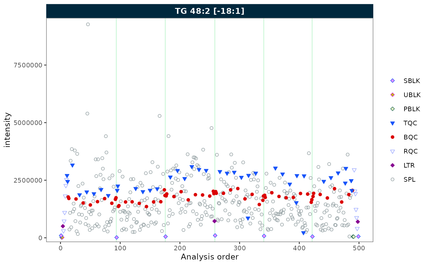

Selecting QC types

Use qc_types to display only specific sample types.

plot_runscatter(mexp, variable = "intensity",
                include_feature_filter = "TG 48\\:2 \\[\\-18:1\\]",
                qc_types = c("BQC", "SPL"),
                rows_page = 1, cols_page = 1)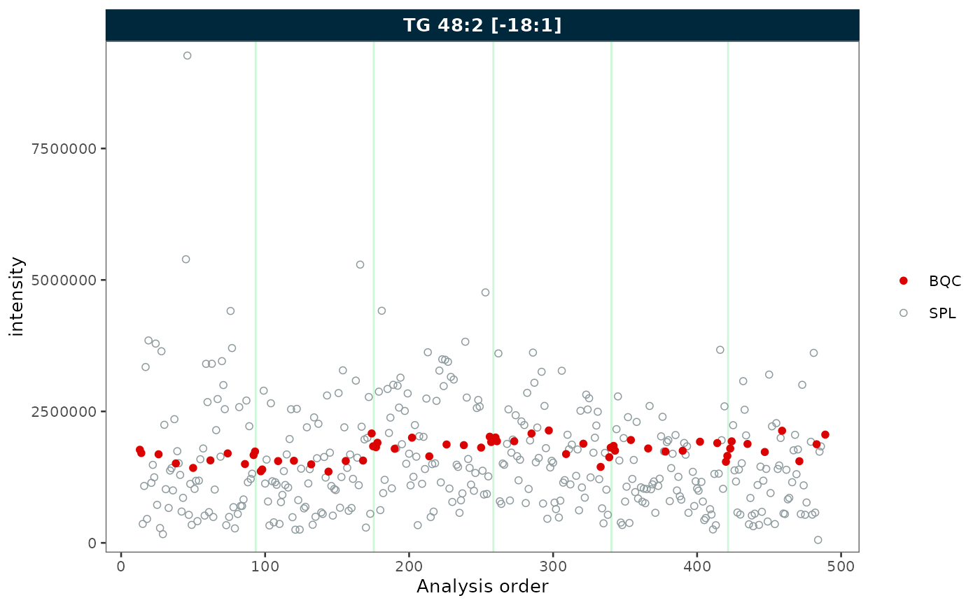

Batch display

Set show_batches = TRUE and batch_zebra_stripe = TRUE to highlight batch boundaries with alternating shaded areas.

plot_runscatter(mexp, variable = "intensity",
                include_feature_filter = "TG 48\\:2 \\[\\-18:1\\]",
                show_batches = TRUE,
                batch_zebra_stripe = TRUE,
                rows_page = 1, cols_page = 1)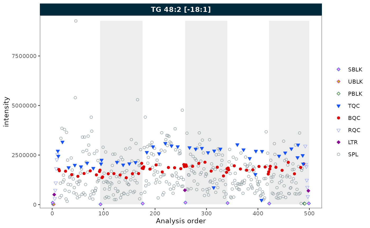

Reference lines

Show mean ± k × SD reference lines with show_reference_lines = TRUE. Use reference_sd_shade to display the range as a shaded band instead of lines.

plot_runscatter(mexp, variable = "intensity",
                include_feature_filter = "TG 48\\:2 \\[\\-18:1\\]",
                qc_types = c("BQC", "SPL"),
                show_reference_lines = TRUE,
                ref_qc_types = "BQC",
                reference_k_sd = 2,
                reference_sd_shade = TRUE,
                rows_page = 1, cols_page = 1)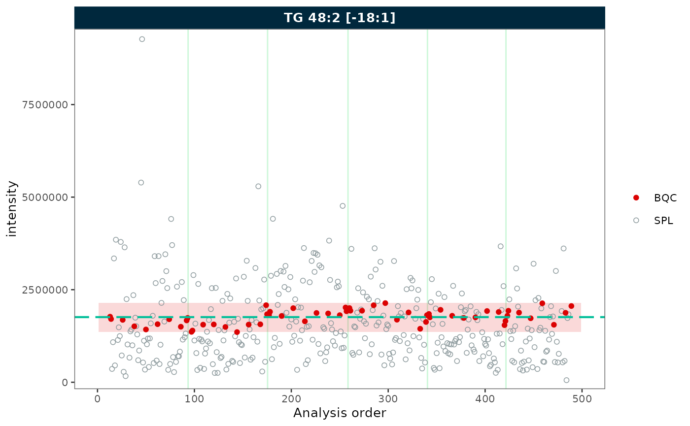

Outlier capping

Use cap_outliers = TRUE to cap extreme values based on MAD fences. This is useful when outliers obscure the trends of QC or study samples.

plot_runscatter(mexp, variable = "intensity",
                include_feature_filter = "TG 48\\:2 \\[\\-18:1\\]",
                cap_outliers = TRUE,
                cap_sample_k_mad = 3,
                rows_page = 1, cols_page = 1)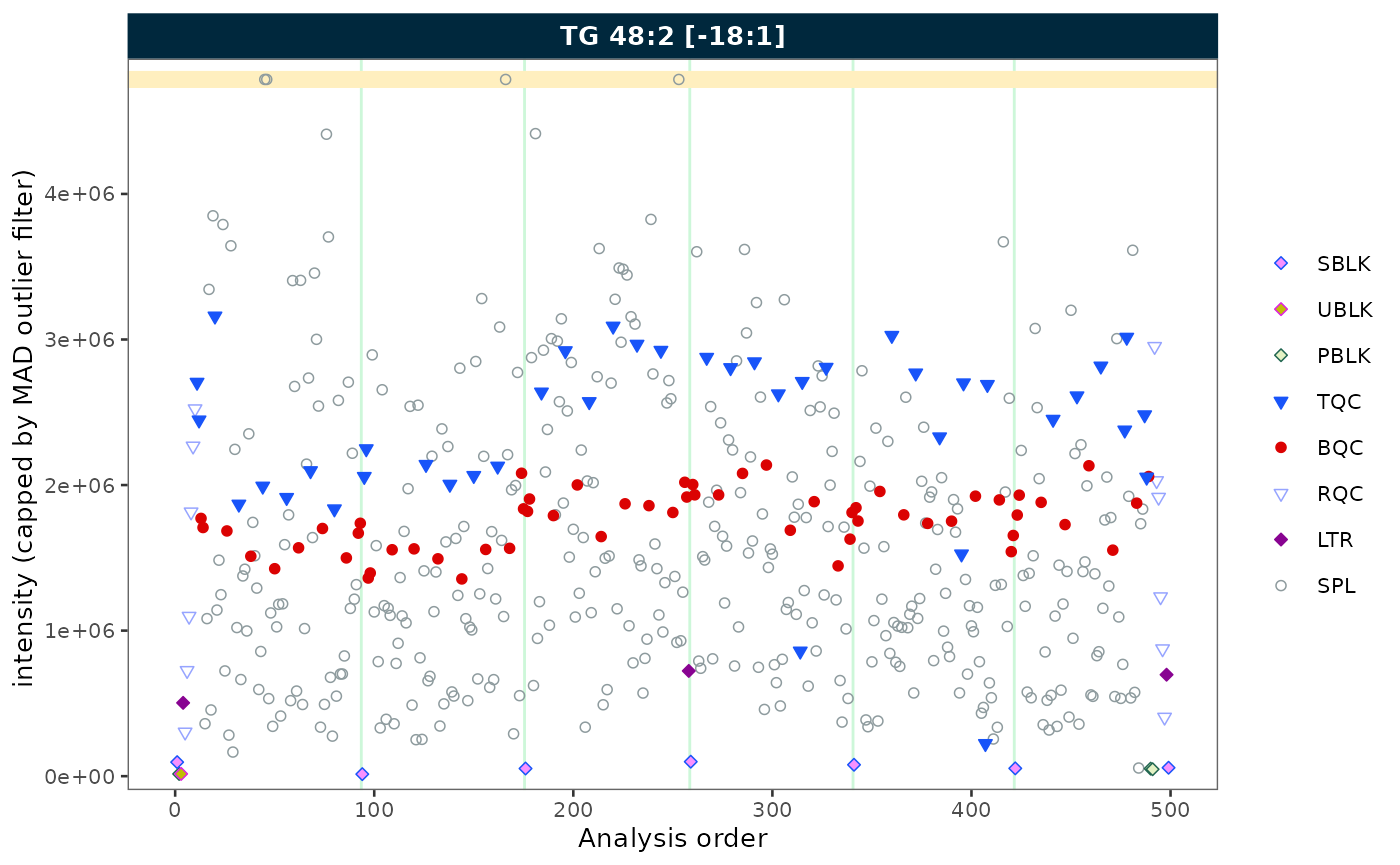

Log scale

Set log_scale = TRUE to apply a log10 transformation to the y-axis. Zero or negative values are replaced with the minimum positive value divided by 5.

plot_runscatter(mexp, variable = "intensity",
                include_feature_filter = "TG 48\\:2 \\[\\-18:1\\]",
                log_scale = TRUE,
                rows_page = 1, cols_page = 1)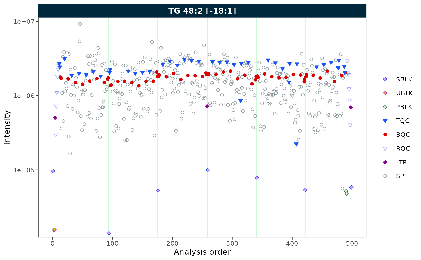

Removing gaps in the analysis sequence

Gaps in the x-axis can arise in two ways:

1. Filtered QC types — when only a subset of QC types is selected, the unselected positions leave gaps. Use collapse_excluded = TRUE to close them.
2. Unannotated analyses — when some runs in the analytical sequence have no corresponding entry in @dataset (e.g. solvent blanks or system suitability injections that were not imported), the analysis order contains discontinuities. Use remove_gaps = TRUE to collapse these and mark the former gap positions with vertical indicator lines.

Both options can be combined.

Collapsing excluded QC types

plot_runscatter(mexp, variable = "intensity",
                include_feature_filter = "TG 48\\:2 \\[\\-18:1\\]",
                qc_types = c("LTR"),
                collapse_excluded = TRUE,
                rows_page = 1, cols_page = 1)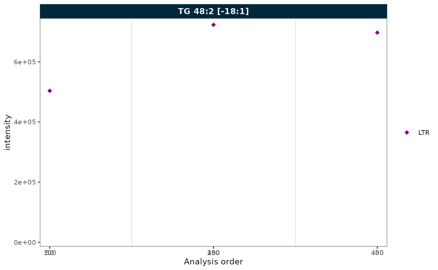

Removing gaps from unannotated analyses

To demonstrate this feature, we first simulate a dataset with unannotated analyses by excluding a block of runs from batch 2. This creates a contiguous gap in the analysis order, as would occur when solvent blanks or system suitability injections are not imported.

mexp_gaps <- exclude_analyses(
  mexp,
  analyses = c(
    paste0("Longit_batch2_", 1:45),
    "Longit_batch2_PQC 12",
    "Longit_batch2_PQC 13",
    "Longit_batch2_PQC 14",
    "Longit_batch2_PQC 15",
    "Longit_batch2_TQC13",
    "Longit_batch2_TQC14",
    "Longit_batch2_TQC15"
  ),
  clear_existing = TRUE
)
mexp_gaps <- normalize_by_istd(mexp_gaps)
mexp_gaps <- calc_qc_metrics(mexp_gaps)

plot_runscatter(mexp_gaps, variable = "intensity",
                include_feature_filter = "TG 48\\:2 \\[\\-18:1\\]",
                remove_gaps = TRUE,
                rows_page = 1, cols_page = 1)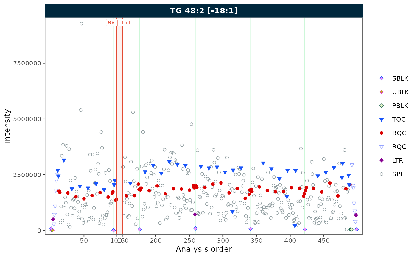

Combining both

When filtering to a single QC type and the sequence contains unannotated runs, combine collapse_excluded and remove_gaps to produce a compact, fully annotated plot.

plot_runscatter(mexp_gaps, variable = "intensity",
                include_feature_filter = "TG 48\\:2 \\[\\-18:1\\]",
                qc_types = c("BQC"),
                collapse_excluded = TRUE,
                remove_gaps = TRUE,
                rows_page = 1, cols_page = 1)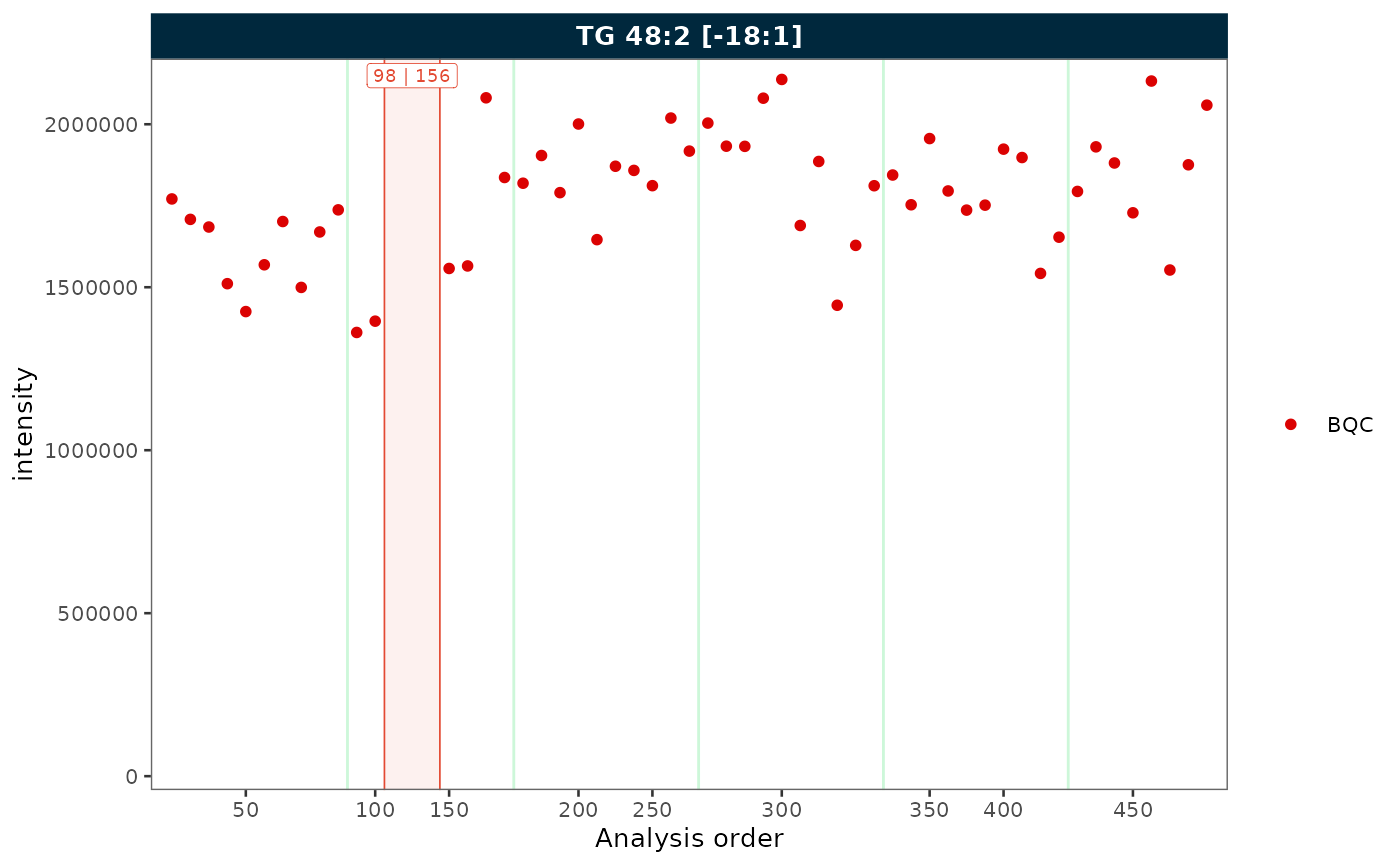

Label wrapping

When feature names are long, strip labels can overflow. Set label_wrap = TRUE to wrap labels across multiple lines, controlled by label_wrap_width. Here we show three features to illustrate the effect on strip text.

plot_runscatter(mexp, variable = "intensity",
                include_feature_filter = "TG 48\\:2 \\[\\-18:1\\]",
                rows_page = 1, cols_page = 3,
                specific_page = 1,
                label_wrap = TRUE,
                label_wrap_width = 8)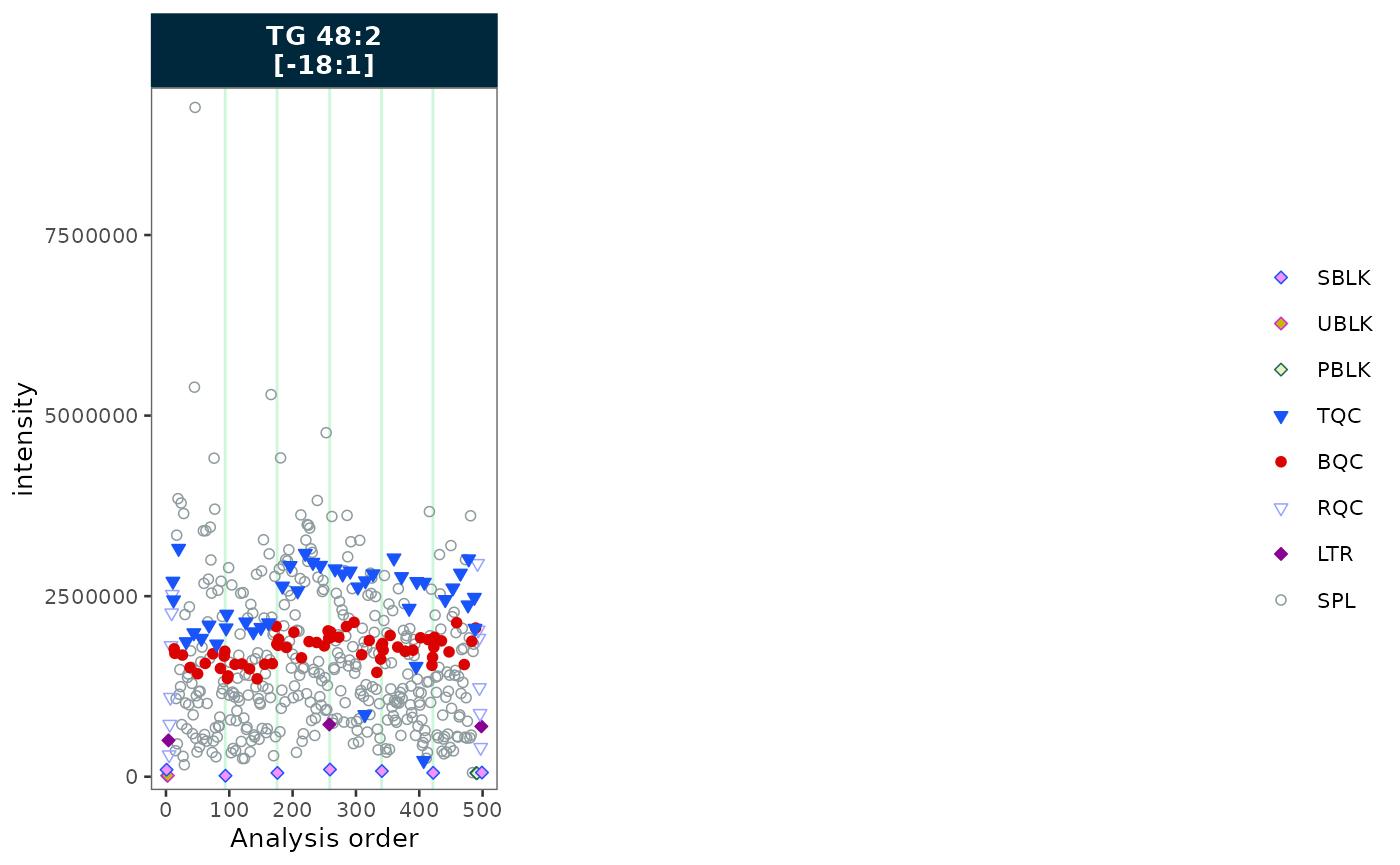

Trend curves

Trend curves visualise the fitted signal used during drift or batch correction. They require a prior correction step — show_trend = TRUE will error if no drift or batch correction has been applied. To plot the values before the last correction, append _before to the variable name (e.g. variable = "intensity_before"); for the original uncorrected values use _raw (e.g. variable = "intensity_raw").

See the Drift Correction tutorial for a worked example.