if (!require("pak")) install.packages("pak")
# This site was rendered with mrmhub 0.9.9 (the QUANT module of MRMhub),
# installed from its default branch (main).
pak::pak("SLINGhub/MRMhub")

# Parallel processing (mirai), coloured console output (fansi), and the
# optional plotting packages used by some QC figures in this workflow.
pak::pak(c("mirai", "fansi", "ggvenn", "patchwork", "ggbeeswarm"))MRMhub Data Processing Workflow for Dataset 3
DYNAMO
1 Overview Dataset
The data come from a human plasma lipidomics study aimed at identifying plasma lipid biomarkers of rapid renal function decline in patients with type 2 diabetes, part of the Diabetes StudY in Nephropathy And other Microvascular cOmplications (DYNAMO) project (Chen et al. (2025)). The lipidomics analysis followed the method of Huynh et al. (2019) with minor modifications, using the same QC sample types as Dataset 1, with the addition of NIST samples. This dataset covers the largest of the study’s four patient cohorts: raw MS data for samples collected at the National University Hospital, Singapore, comprising 3,816 plasma samples and 775 blank and QC samples (4,591 in total). In total, 748 MRM transitions were monitored, from which 828 features were integrated. For the biological and clinical conclusions related to these data, we refer readers to the original publication (Chen et al. 2025).
This example workflow covers the complete MRMhub data processing pipeline on this dataset: peak integration, quantitation, quality control and reporting. It includes many elements of the MRMhub workflow, some of which may not be applicable or necessary for other datasets.
ImportantData availability
All code and data for this workflow are deposited in the Zenodo record 10.5281/zenodo.15370293 (MRMhub-workflows). The corresponding MS raw data (mzML files), together with the MRMhub-INTEGRATOR application and its input files, are deposited as MRMhub-Dataset3.zip in the same record.
2 Raw Data Processing: Peak Picking and Integration
Peak picking and peak integration were performed with MRMhub-INTEGRATOR; the key aspects for this dataset are given below. For a more detailed description of the workflow, see Workflow for Dataset 1 and the INTEGRATOR Manual.
2.1 Conversion of vendor raw files to mzML
The original raw data files (Agilent .d) were converted to mzML using msconvert from the ProteoWizard software (https://proteowizard.sourceforge.io) with the following settings: output format = mzML; binary encoding precision = 32 bit; write index = true.
2.2 Preparation of the INTEGRATOR input files
The final input files used for this dataset are contained in MRMhub-Dataset3.zip (see above), for those who wish to re-run the integration. The following subsections summarize the key settings used for this example.
2.2.1 Global Settings File (param.txt)
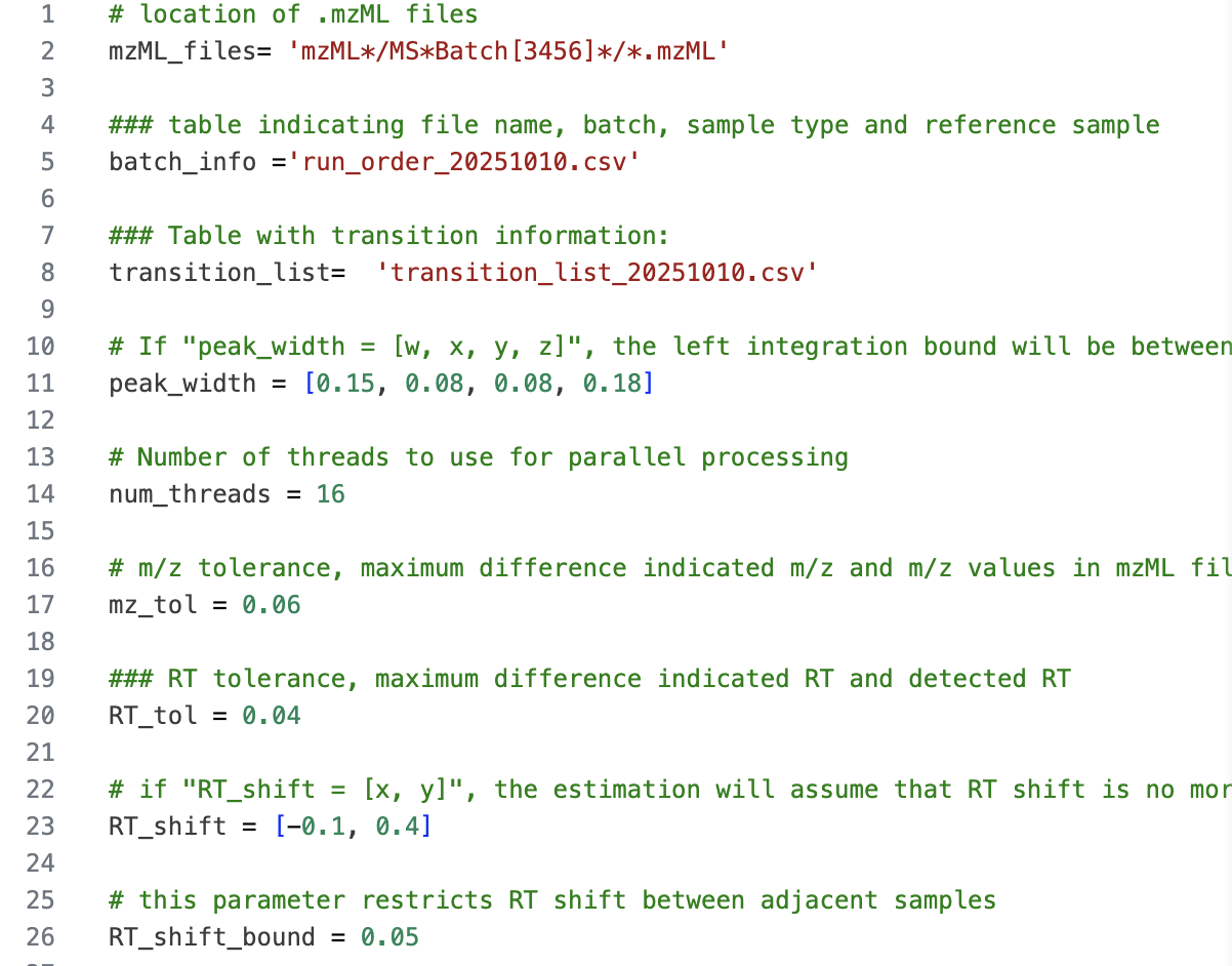
The parameter mz_tol, defining the maximum tolerance in m/z values for identifying transitions, was set to 0.06. The RT_tol parameter, defining the window around the expected RT (see Feature/Transition table below) in which features are searched, was set to 0.04 min. This relatively narrow RT window was chosen to reduce selection of incorrect peaks in complex chromatograms, as observed in this dataset. The global peak_width parameter was set to [0.15, 0.08, 0.08, 0.18], which matched the majority of the peaks. For specific features with broader or convoluted peaks, feature-specific peak widths were applied, overwriting the global settings (see Feature Table below). The maximum allowed RT shift correction was set to (-0.1, 0.4), and the maximum allowed sample-to-sample RT shift was 0.05 min. The full set of settings in param.txt is shown in the figure below.
2.2.2 Sample Table
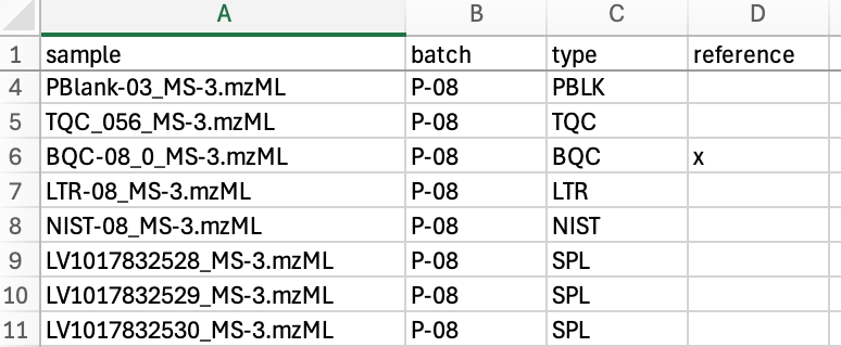
In the sample table (run_order_20251010.csv) the samples to be processed were listed by their .mzML file names. The first two BQC (batch quality control) samples were selected as retention time reference anchors. The sample type for each sample was defined in column C (sample_type) using the MRMhub QC type nomenclature. This is optional and INTEGRATOR distinguishes only between blanks (identified by the presence of the text BLK), and non-blanks.
2.2.3 Feature/Transition (Feature) Table
The feature/transition table (transition_list_20251010.csv) defined the transitions to be extracted from the .mzML files by precursor and product m/z values. Each feature (peak or peak group) was specified by its expected retention time (RT, in minutes). For some transitions, multiple features were defined. The corresponding internal standard feature for each entry was included in the table, however, these internal standards were not used by INTEGRATOR but were exported in the integration results.
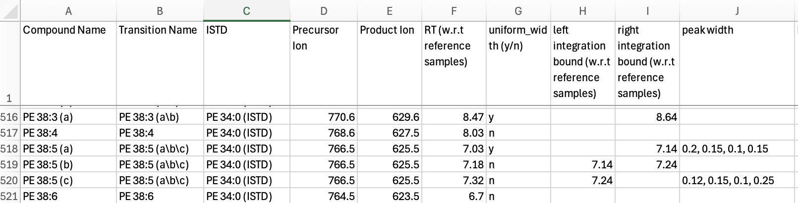
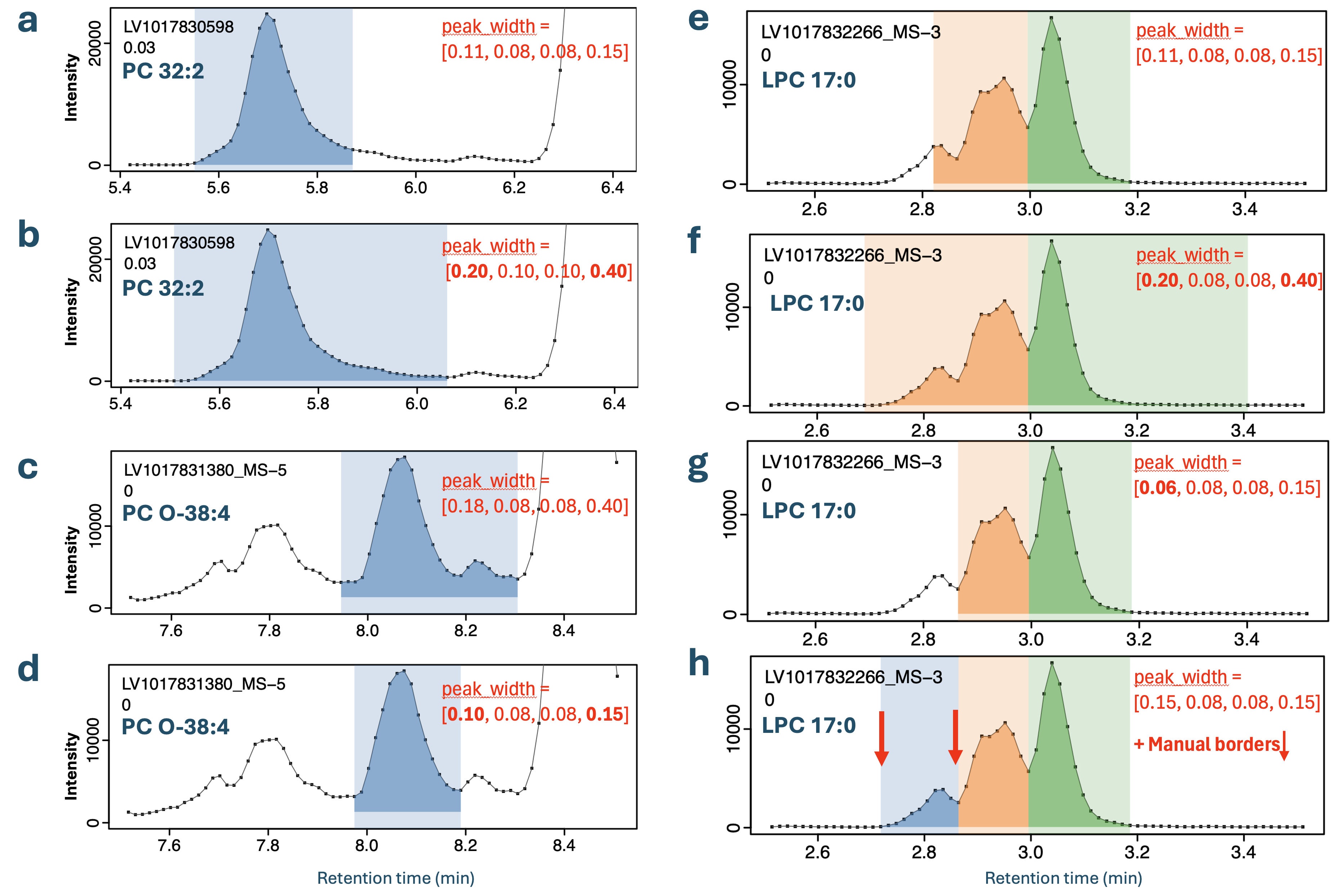
Feature-specific ‘peak_width’ settings were applied for multiple features in this dataset when peaks were broader, exhibited increased tailing, or consisted of convoluted peaks that had to be co-integrated (see Figure 4 a-d). Fixed borders were assigned for features for which automatic integration failed or produced inconsistent results due to being poorly separated from adjacent peaks or having noisy chromatograms (see Figure 4 e-h). The final version of the feature/transition table (transition_list_20251010_Final.csv) is the result from several rounds of parameter optimization with INTEGRATOR.
2.3 Running MRMhub-INTEGRATOR and Review of Results
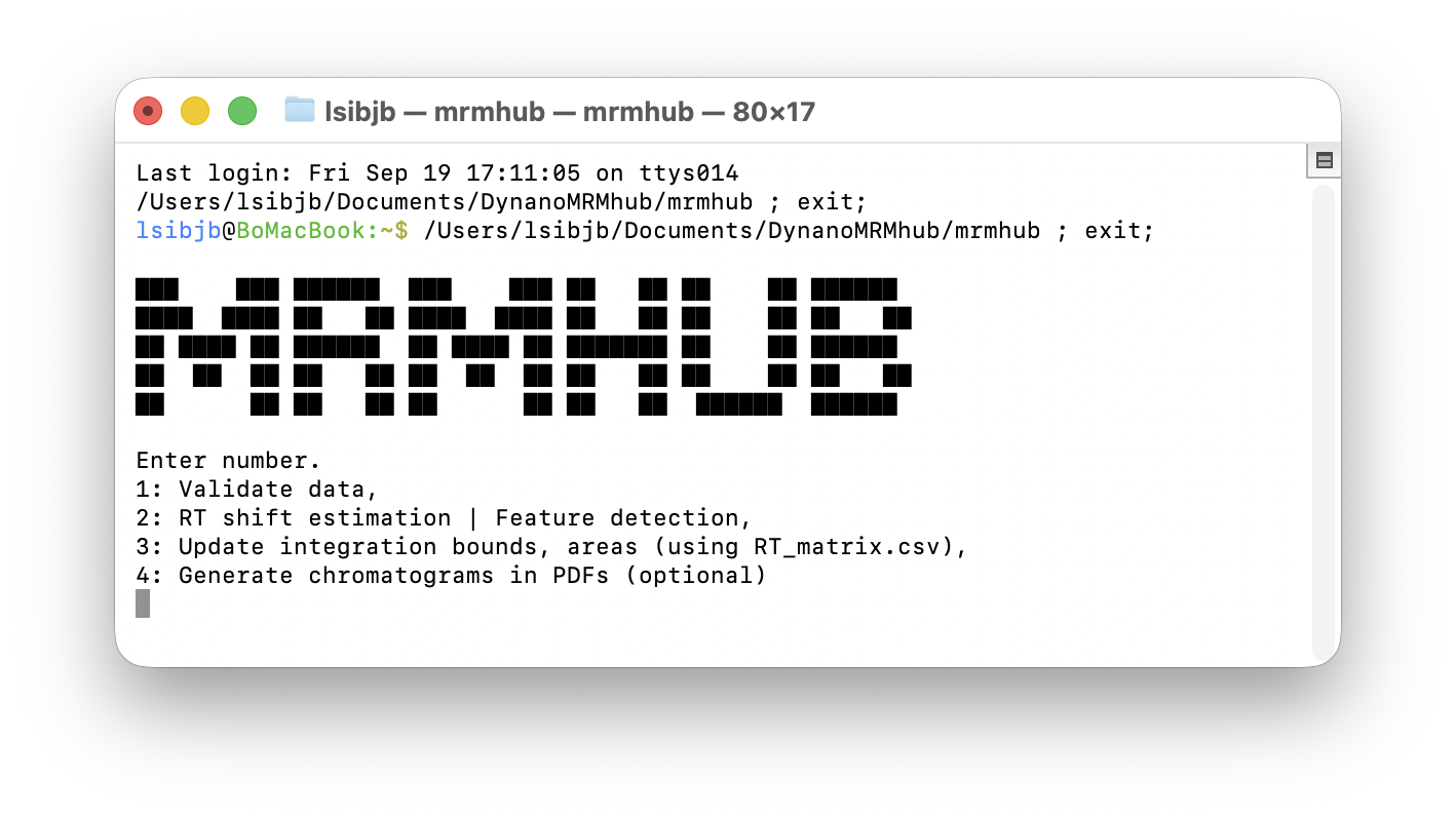
The most recent release of INTEGRATOR was obtained from https://github.com/SLINGhub/MRMhub/releases. After preparing all input files, the INTEGRATOR application is started. Steps 1 to 4 then run consecutively without further input to perform peak detection, peak picking, integration, and export of data and PDF results. The integration results are reported in the generated file ‘long.csv’, a long-format table that includes peak areas, actual retention time, peak width, and other metadata. This data file will be used for subsequent data postprocessing (see the following section). A wide-format table with peak areas is available as ‘quant_raw.csv’. PDFs of the integrated transitions are available in the by_* folders. See the INTEGRATOR Manual for more details.
The peak integration results were inspected for all features across samples using the generated PDFs (see above). In this dataset, RT shifts across the entire run of 4,591 samples were less than 0.04 min, except for ~ 20 samples at the start of a batch towards the end of this analysis, which had increased RT shifts.
3 Data Postprocessing and QC
3.1 Setting up a Quarto Notebook and Installation of {mrmhub}
A Quarto notebook was created in RStudio. The {mrmhub} R package was installed by running the following code in the R console, together with the mirai (parallel processing) and fansi (coloured console output) packages, and the optional plotting packages (ggvenn, patchwork, ggbeeswarm) used in this workflow.
Notemrmhub version
These notebooks were rendered with mrmhub 0.9.9 (QUANT module of MRMhub, main branch); install with pak::pak("SLINGhub/MRMhub").
The Quarto notebook code generated in this example workflow is available from https://github.com/SLINGhub/MRMhub-workflows (file Dataset3.qmd). In the subsequent section, the data postprocessing is encoded and documented step-by-step into the notebook as individual code chunks using {mrmhub} functions.
3.2 Postprocessing workflow
3.2.1 Load mrmhub and other required R packages
To improve performance, multi-threading was used for some of the calculations and plotting, for which the R package {mirai} needs to be installed and loaded.
library(mrmhub)

# Colour mrmhub's cli console feedback in the rendered HTML (requires the fansi package)
mrmhub_enable_cli_color()

# --- Optional: multithreading -------------------------------------------------
# This workflow runs single-threaded by default, so it renders with only the
# packages installed alongside mrmhub. Some steps -- plot_runscatter() PDF export
# and drift/batch correction -- can run in parallel for a substantial speed-up,
# which requires the mirai, carrier and qpdf packages. To enable it, install them
# once with:
#   pak::pak(c("mirai", "carrier", "qpdf"))
# then uncomment the two lines below and set multithreading = TRUE in the
# plot_runscatter() calls further down.
# n_cores <- max(1L, {n <- parallel::detectCores(); if (is.na(n)) 4L else n} - 1L)
# if (mirai::status()$daemons == 0) mirai::daemons(n_cores)
NoteOptional: multithreading
This workflow runs single-threaded by default, so it renders with only the packages installed alongside mrmhub. Some steps — plot_runscatter() PDF export and drift/batch correction — can run in parallel for a substantial speed-up. This requires three additional packages:
pak::pak(c("mirai", "carrier", "qpdf"))Once installed, uncomment the mirai daemon setup in the setup chunk above and set multithreading = TRUE in the plot_runscatter() calls.
3.2.2 Import the MRMhub-INTEGRATOR results
The results from the peak integration performed with the INTEGRATOR workflow, as described in the previous section, were imported into a MRMhubExperiment data object. This object represents the central data container used in this postprocessing workflow. The original result file from INTEGRATOR (‘long.csv’) has been renamed to ‘Dataset3_MRMhub-INTEGRATOR_Final.csv’.
data_path <- "./data/dataset-3/Dataset3_MRMhub-INTEGRATOR_Final.csv"
mexp <- MRMhubExperiment()
mexp <- import_data_mrmhub(mexp, data_path, import_metadata = TRUE)
✔ Imported 4591 analyses with 828 features.ℹ feature_area selected as default feature intensity. Modify with `set_intensity_var()`.✔ Analysis metadata associated with 4591 analyses.✔ Feature metadata associated with 828 features.3.2.3 Import the analysis metadata
Detailed analysis metadata, describing the analytes, samples, features, internal standards (ISTDs), and response curves required for subsequent steps, were imported from the Excel workbook ‘Dataset3_Metadata.xlsx’, included in this repository under data/dataset-3/.
file_path <- "./data/dataset-3/Dataset3_Metadata.xlsx"
mexp <- import_metadata_msorganiser(mexp, file_path, ignore_warnings = TRUE)
#> Found no errors, 1 warning, and no notes in the metadata.
#> -----------------------------------------------------------------
#>   Type  Table    Column     Issue                           Count
#> 1 W*    Features feature_id Feature(s) not in analysis data    30
#>
#> -----------------------------------------------------------------
#> E = Error, W = Warning, W* = Suppressed Warning, N = Note
#> -----------------------------------------------------------------
✔ Analysis metadata associated with 4591 analyses.✔ Feature metadata associated with 828 features.✔ Internal Standard metadata associated with 26 ISTDs.✔ Response curve metadata associated with 36 annotated analyses.3.2.4 Analytical design and timeline
An overview of the analysis structure, detailing the types and sequence of QC samples analyzed is provided by the plot below. It also shows information on the start and end dates, total duration, and median run time for each sample. The last four batches were measured approximately one year after the others.
plot_runsequence(
  mexp,
  show_batches = TRUE,
  qc_types = c(
    "SPL",
    "BQC", "TQC", "PBLK", "UBLK", "RQC", "SBLK", "LTR", "NIST"),
  batch_zebra_stripe = TRUE, font_base_size = 6,
  batch_fill_color = "#fffbdb", segment_linewidth = 0.25,
  show_timestamp = FALSE) +
  theme(plot.title = element_text(size = 5))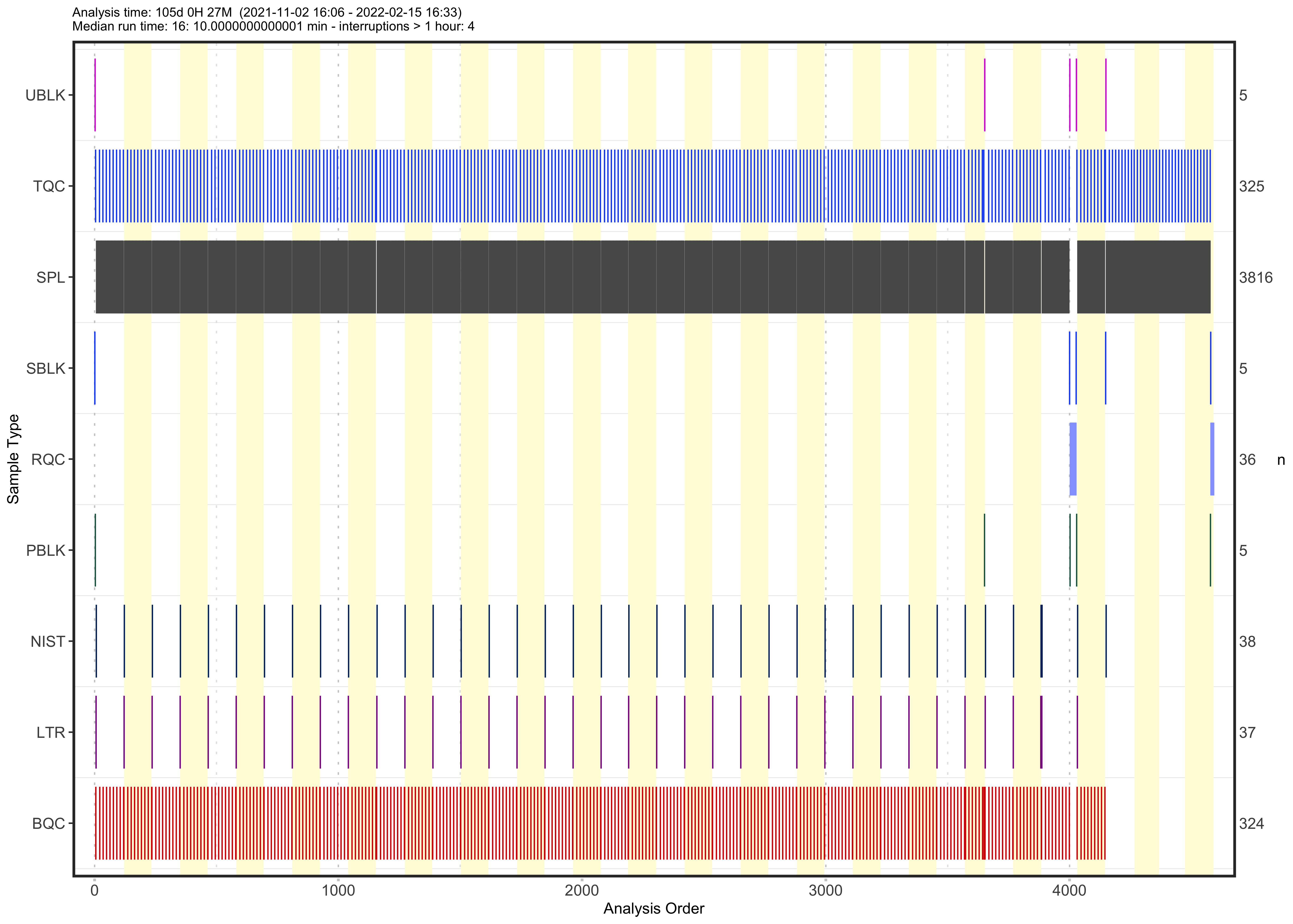
3.2.5 Overview Chromatographic Separation
The following plot shows the retention time distribution of all detected lipid species. The ceramides (Cer) species show little chromatographic separation in contrast to other lipid classes, with the majority eluting between 10.0 to 10.5 min. The triglycerides (TG) also elute within a narrower retention time range at around 11 min.
plot_abundanceprofile(
  data = mexp,
  log_scale = FALSE,
  variable = "rt",
  density_strip = TRUE,
  qc_types = "SPL",
  analysis_range = c(1, 4000),
  show_sum = FALSE,
  #x_lim = c(6.5, 7.5),
  x_label = NA,
  feature_map = "lipidomics")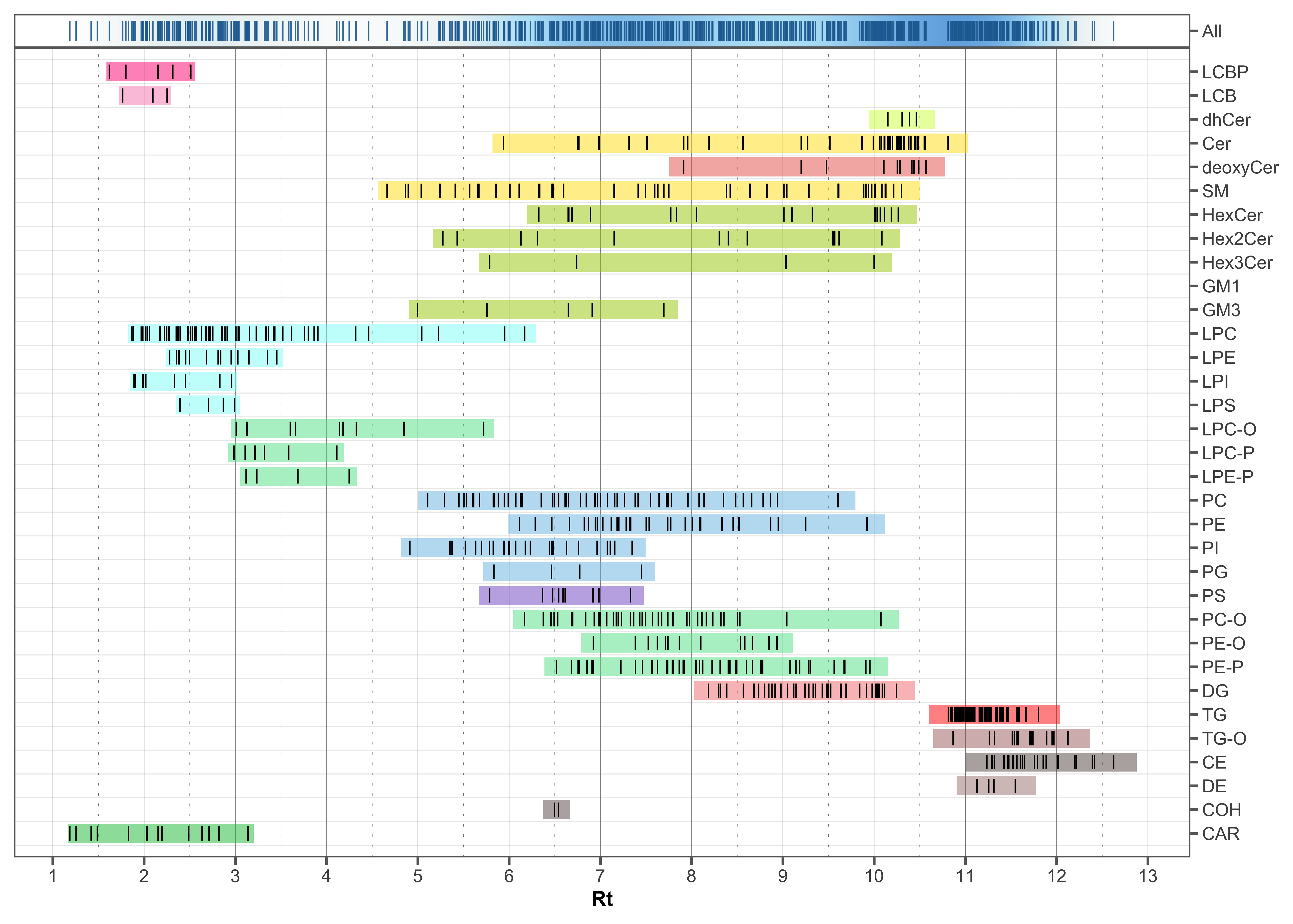
3.2.6 Overall trends and check for possible outliers
To examine overall technical trends and issues affecting most analytes (features), the Relative Log Abundance (RLA) plot is useful (De Livera et al. 2012; Livera et al. 2015). In an RLA plot, each feature is normalized to the across-sample or within-batch median and the resulting values are shown as boxplots for each sample. This visualization helps identify technical problems such as pipetting errors, sample loss, or changes in injection volume or instrument sensitivity. First, an overview of all analyses is plotted, showing only the signals from the spiked-in internal standards (ISTDs); the red horizontal lines indicate the 1.5× IQR outlier limits.
fig2a <- plot_rla_boxplot(
  data = mexp,
  rla_type_batch = c("within"),
  variable = "intensity",
  qc_types = c("BQC", "TQC", "SPL", "NIST", "LTR", "SBLK"),
  #plot_range = c(1, 4900),
  rla_limit_to_range = FALSE,
  filter_data = FALSE,
  min_feature_intensity = 1000,
  include_feature_filter = "ISTD",
  #y_lim = c(-4,4),
  show_timestamp = FALSE, outlier_method = "fold", outlier_k = c(-0.4, 0.3),
  outlier_exclude = FALSE, x_gridlines = FALSE, show_plot = TRUE,
  batch_zebra_stripe = TRUE, linewidth = 0.1)
ℹ Found 148 outliers in the 4545 shown analyses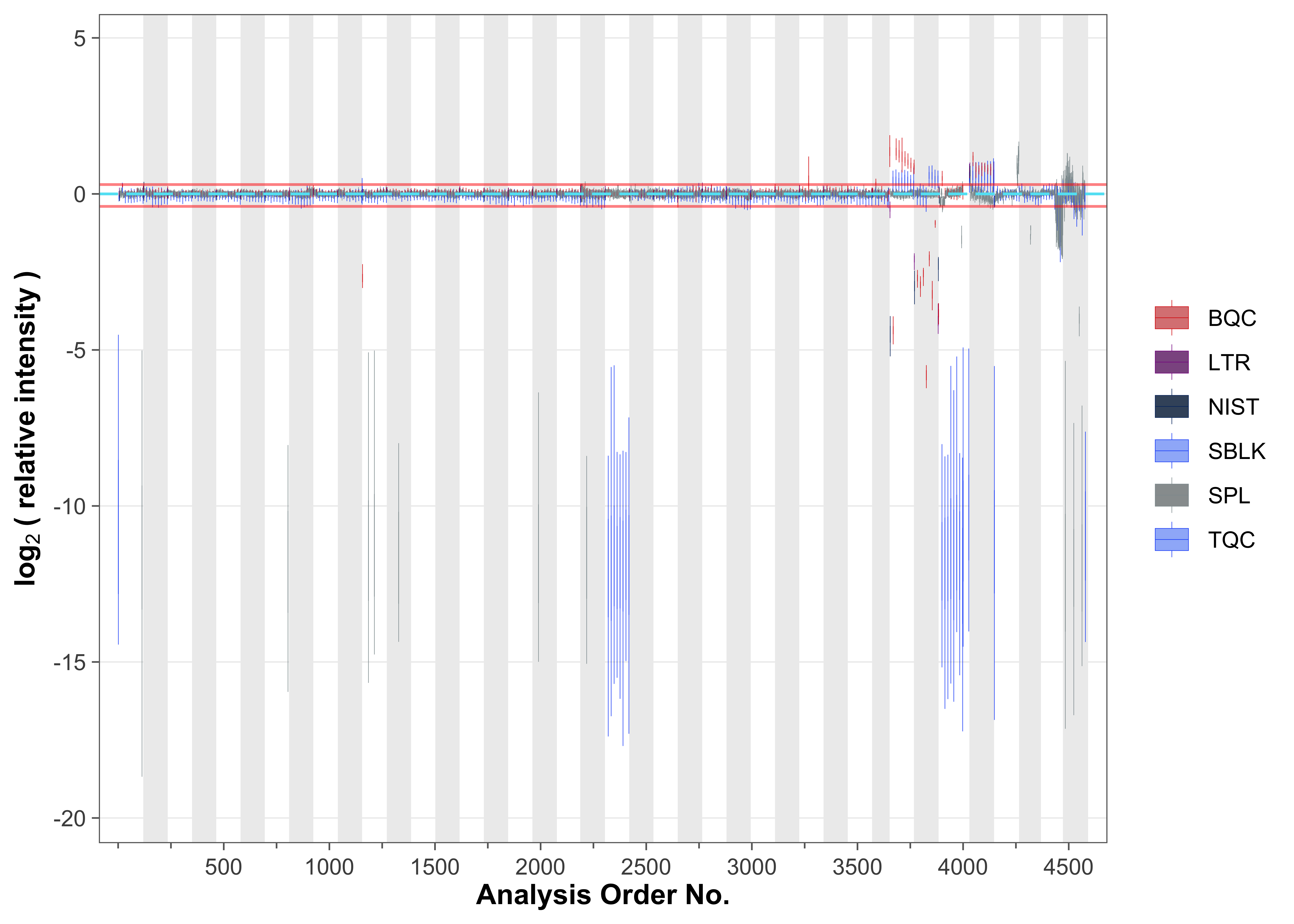
Several outliers among study and QC samples were detected using this RLA analysis (visible also in the plot above).
# Get outlier in ISTD total signal excluding 3 batches with overall lower ISTD
istd_outlier <- fig2a$outliers |>
filter(!(batch_id %in% c("P-01", "P-02", "P-43") & val_res_median > -3))
print(istd_outlier)
#> [38;5;246m# A tibble: 79 × 5[39m
#> analysis_id analysis_order batch_id val_res_median qc_type
#> [3m[38;5;246m<chr>[39m[23m [3m[38;5;246m<int>[39m[23m [3m[38;5;246m<chr>[39m[23m [3m[38;5;246m<dbl>[39m[23m [3m[38;5;246m<chr>[39m[23m
#> [38;5;250m 1[39m LV1017832619_MS-3 113 P-08 -[31m11[39m[31m.[39m[31m9[39m SPL
#> [38;5;250m 2[39m LV1017835020_MS-3 804 P-14 -[31m11[39m[31m.[39m[31m7[39m SPL
#> [38;5;250m 3[39m BQC-18_0_MS-4 [4m1[24m157 P-18 -[31m2[39m[31m.[39m[31m68[39m BQC
#> [38;5;250m 4[39m LV1017831110_MS-4 [4m1[24m185 P-18 -[31m11[39m[31m.[39m[31m7[39m SPL
#> [38;5;250m 5[39m LV1017832095_MS-4 [4m1[24m213 P-18 -[31m11[39m[31m.[39m[31m6[39m SPL
#> [38;5;250m 6[39m LV1017831999_MS-4 [4m1[24m328 P-19 -[31m11[39m[31m.[39m[31m8[39m SPL
#> [38;5;250m 7[39m LV1017834759_MS-4 [4m1[24m990 P-25 -[31m11[39m[31m.[39m[31m9[39m SPL
#> [38;5;250m 8[39m LV1017834663_MS-5 [4m2[24m218 P-27 -[31m11[39m[31m.[39m[31m4[39m SPL
#> [38;5;250m 9[39m TQC_217_MS-5 [4m2[24m320 P-28 -[31m12[39m[31m.[39m[31m0[39m TQC
#> [38;5;250m10[39m TQC_218_MS-5 [4m2[24m334 P-28 -[31m12[39m[31m.[39m[31m7[39m TQC
#> [38;5;246m# ℹ 69 more rows[39mTo confirm these potential outliers, the peak areas of all ISTDs in different QC types are plotted against the run order (RunScatter plot). The outliers seen in these plots (with values close to zero) correspond to the outliers seen in the RLA plot above.
plot_runscatter(
  mexp,
  variable = "intensity",
  include_qualifier = FALSE,
  qc_types = c("SPL", "BQC", "TQC", "PBLK", "RQC", "SBLK"),
  include_feature_filter = "IS",
  #y_min = 0.00, y_max = 0.15,
  #plot_range = c(0, 910),
  point_size = .2, point_border_width = 0.1, point_alpha = .7,
  font_base_size = 4, cols_page = 3, rows_page = 11, show_progress = FALSE,
  cap_outliers = TRUE)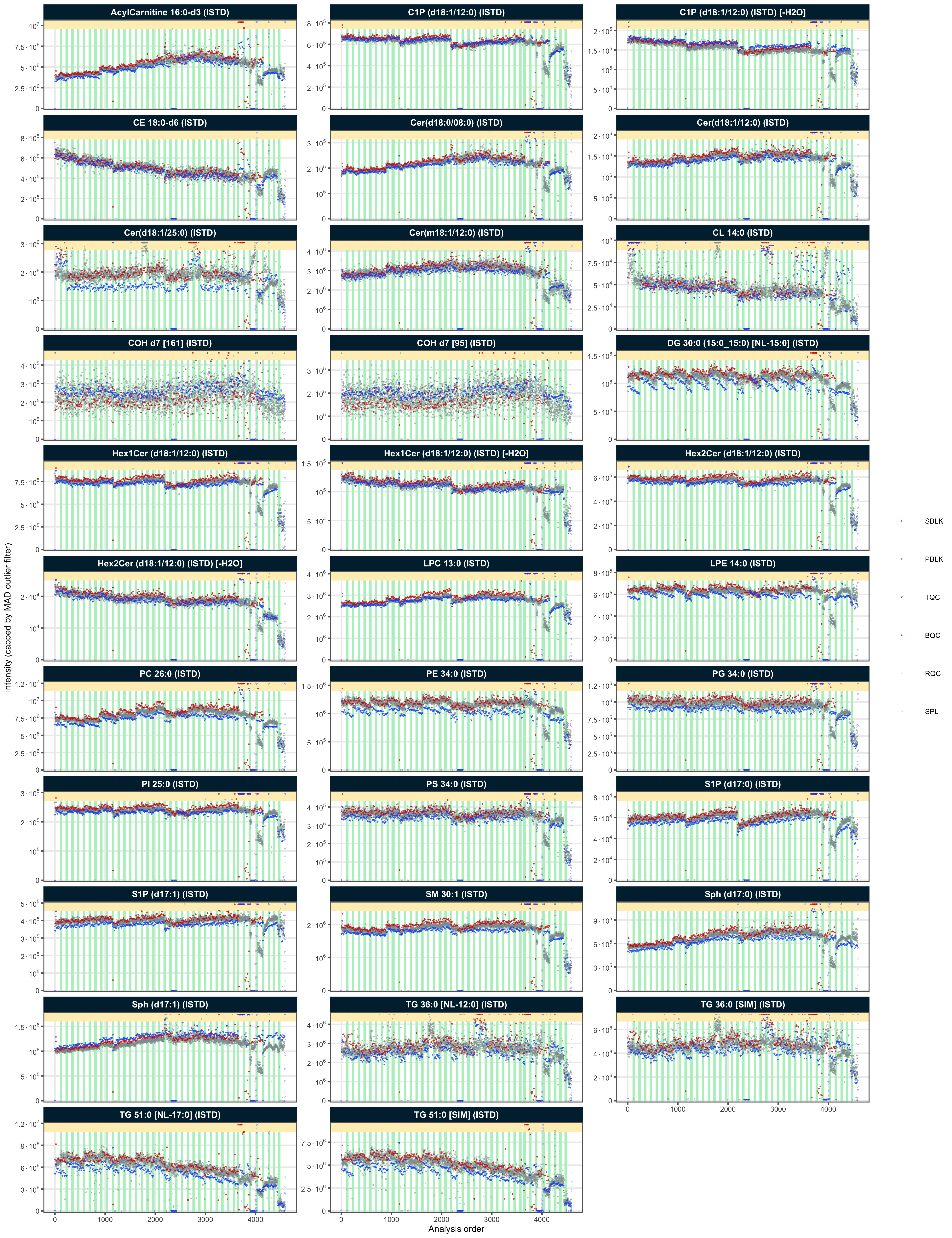
Separately, the full dataset is then checked for potential systematic outliers in endogenous analytes.
fig2b <- plot_rla_boxplot(
  data = mexp,
  rla_type_batch = c("within"),
  variable = "intensity",
  qc_types = c("BQC", "TQC", "SPL", "NIST", "LTR"),
  filter_data = FALSE,
  min_feature_intensity = 1000,
  exclude_feature_filter = "ISTD",
  plot_range = c(1, 4800),
  #y_lim = c(-4,4),
  show_timestamp = FALSE, outlier_method = "fold", outlier_k = c(-2, 1),
  outlier_exclude = FALSE, x_gridlines = FALSE, batch_zebra_stripe = TRUE,
  show_plot = TRUE, linewidth = 0.1)
ℹ Found 80 outliers in the 4540 shown analyses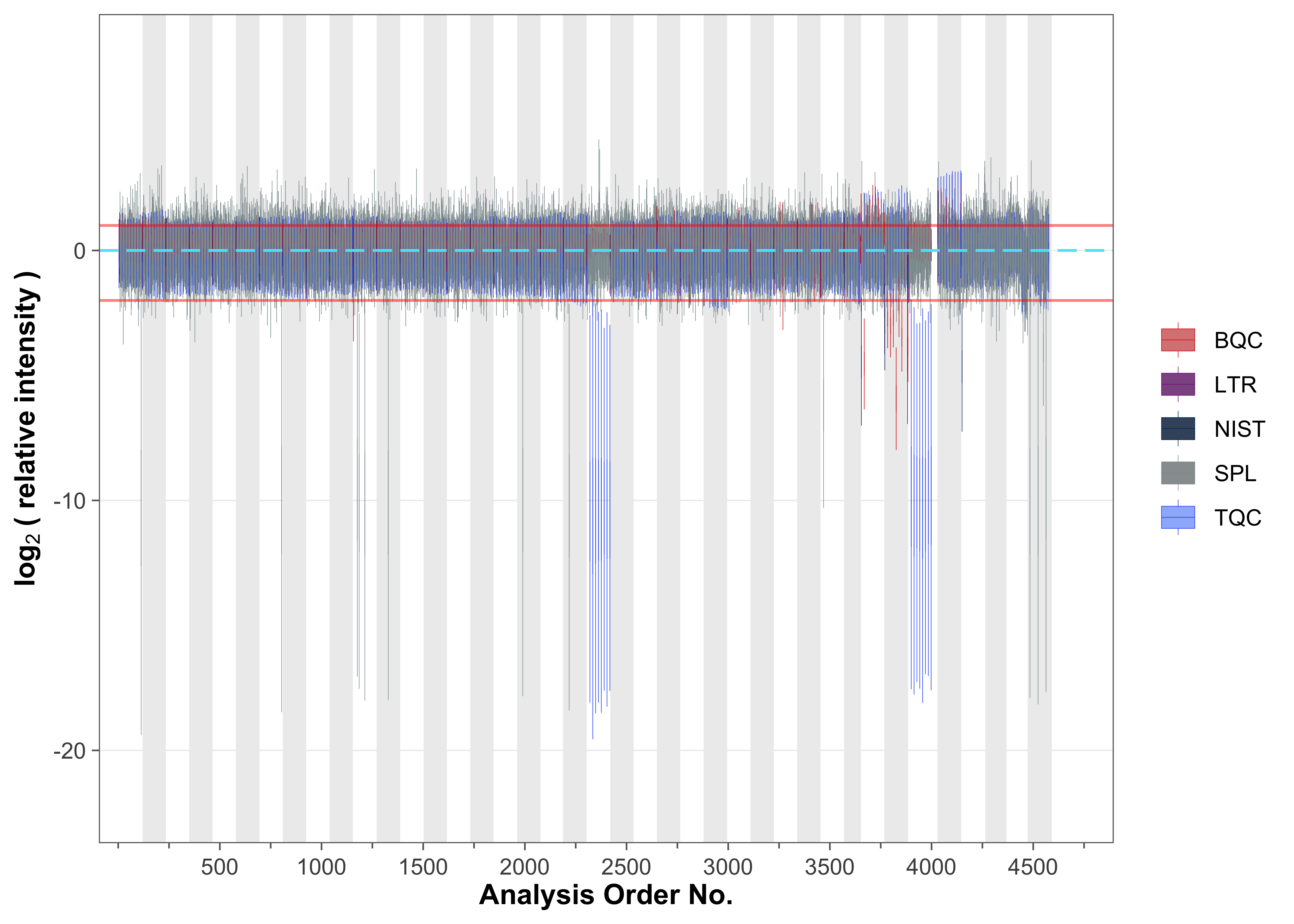
Also for the endogenous analytes, several outliers among study and QC samples were detected:
# Get outliers in the endogenous-analyte signals, excluding the 3 batches with
# consistently lower ISTD
analyte_outlier <- fig2b$outliers |>
filter(!(batch_id %in% c("P-01", "P-02", "P-43") & val_res_median > -3))
print(analyte_outlier)
#> [38;5;246m# A tibble: 72 × 5[39m
#> analysis_id analysis_order batch_id val_res_median qc_type
#> [3m[38;5;246m<chr>[39m[23m [3m[38;5;246m<int>[39m[23m [3m[38;5;246m<chr>[39m[23m [3m[38;5;246m<dbl>[39m[23m [3m[38;5;246m<chr>[39m[23m
#> [38;5;250m 1[39m LV1017832619_MS-3 113 P-08 -[31m10[39m[31m.[39m[31m5[39m SPL
#> [38;5;250m 2[39m LV1017835020_MS-3 804 P-14 -[31m9[39m[31m.[39m[31m89[39m SPL
#> [38;5;250m 3[39m BQC-18_0_MS-4 [4m1[24m157 P-18 -[31m2[39m[31m.[39m[31m29[39m BQC
#> [38;5;250m 4[39m LV1017832063_MS-4 [4m1[24m176 P-18 -[31m9[39m[31m.[39m[31m51[39m SPL
#> [38;5;250m 5[39m LV1017831110_MS-4 [4m1[24m185 P-18 -[31m9[39m[31m.[39m[31m98[39m SPL
#> [38;5;250m 6[39m LV1017832095_MS-4 [4m1[24m213 P-18 -[31m10[39m[31m.[39m[31m0[39m SPL
#> [38;5;250m 7[39m LV1017832134_MS-4 [4m1[24m260 P-18 1.23 SPL
#> [38;5;250m 8[39m LV1017831999_MS-4 [4m1[24m328 P-19 -[31m9[39m[31m.[39m[31m78[39m SPL
#> [38;5;250m 9[39m LV1017834759_MS-4 [4m1[24m990 P-25 -[31m9[39m[31m.[39m[31m81[39m SPL
#> [38;5;250m10[39m LV1017834663_MS-5 [4m2[24m218 P-27 -[31m10[39m[31m.[39m[31m4[39m SPL
#> [38;5;246m# ℹ 62 more rows[39mInspection of the generated plots and outlier tables identified several individual study samples, Technical QC (TQC), and Batch QC (BQC) samples that exhibited markedly lower signals for both internal standards (ISTDs) and endogenous analytes. TQC samples from two batches showed similarly reduced signals, while adjacent samples displayed normal signal levels, suggesting potential issues with sample preparation or errors in the LC-MS worklist for these specific samples and batches. Accordingly, these samples were classified as technical outliers and excluded from subsequent analysis.
Furthermore, in three batches analyzed toward the end of the sequence, all BQC samples exhibited marked differences in ISTD and analyte signals, whereas study samples in the same batch presented normal signals. This pattern is indicative of probable sample preparation errors affecting these BQCs. Consequently, they were also classified as technical outliers and excluded from the dataset.
Finally, an additional 18 samples were identified as outliers based on their endogenous analyte signals, although their ISTD signals remained comparable to other samples. These discrepancies were attributed to errors that occurred during the pipetting of sample aliquots into the extraction tubes.
# Outliers in analyte but not ISTD signals
setdiff(analyte_outlier$analysis_id, istd_outlier$analysis_id)
#>  [1] "LV1017832063_MS-4" "LV1017832134_MS-4" "LV1017834496_MS-5"
#>  [4] "LV1017834500_MS-5" "LV1017831025_MS-5" "BQC-30_8_MS-5"
#>  [7] "BQC-31_0_MS-5"     "LV1017831362_MS-5" "BQC-34_4_MS-5"
#> [10] "BQC-36_2_MS-5"     "BQC-37_5_MS-5"     "BQC-37_7_MS-5"
#> [13] "LV1017834075_MS-5" "LV1017832625_MS-5" "LV1017832682_MS-5"
#> [16] "NIST-04"           "LV1017830587"      "LV1017830728"
In total, 98 analyses/samples were classified as technical outliers and are excluded from further analysis.
# Combined ISTD and analyte outlier
outlier_combined <- istd_outlier |>
  bind_rows(analyte_outlier) |>
  bind_rows(tibble(analysis_id = "NIST-04", qc_type = "NIST")) |>
  select(-val_res_median) |>
  distinct()

outlier_combined |> dplyr::count(qc_type)
mexp <- exclude_analyses(
  mexp,
  analyses = outlier_combined$analysis_id, clear_existing = TRUE)
✔ 97 analyses were excluded for downstream processing. Please reprocess data.To check that these outliers were removed, the ISTDs are plotted again. The ISTD signals were fairly stable in the first 35 batches, then varied in the last 4 batches.
plot_runscatter(
  mexp,
  variable = "intensity",
  include_qualifier = FALSE,
  qc_types = c("SPL", "BQC", "TQC", "PBLK", "RQC", "SBLK"),
  include_feature_filter = "IS",
  #y_min = 0.00, y_max = 0.15,
  #plot_range = c(0, 910),
  point_size = .2, point_border_width = 0.1, point_alpha = .7,
  font_base_size = 4, cols_page = 3, rows_page = 11, show_progress = FALSE,
  cap_outliers = TRUE)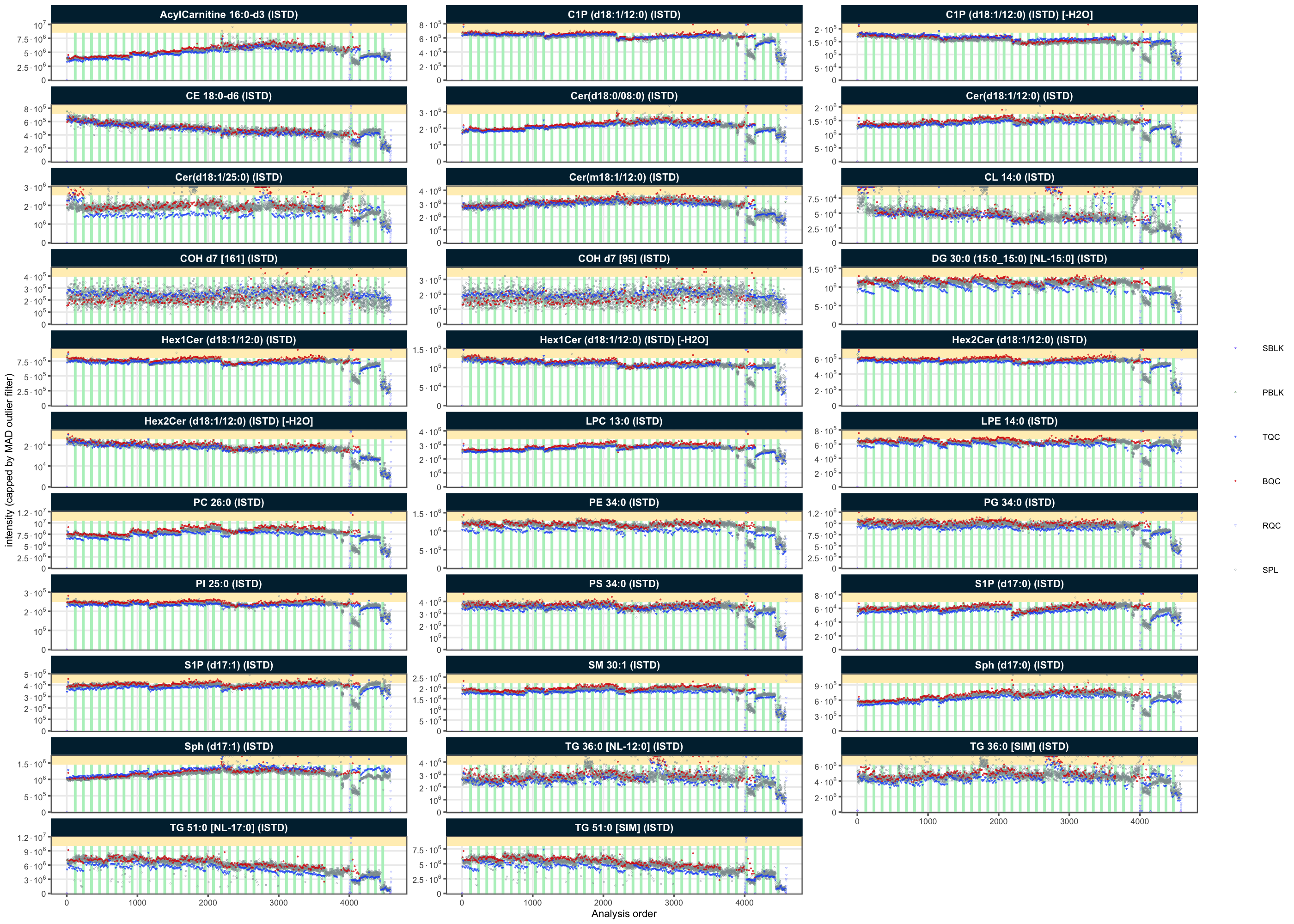
3.3 Peak picking QC
To check for potential peak picking errors, the retention time (RT) of lipid features was plotted against the total carbon number and the number of double bonds in the acyl chains. This dataset was the result of an iterative process involving data review with QC plots and curation, which removed detectable annotation errors. Lipid species that remained flagged as potential misannotations were then manually inspected in the chromatograms and compared with an online resource providing peak annotation information for the utilized LC-MS method (https://metabolomics.baker.edu.au/method/lipids). Following this verification, these features were deemed likely to be correct.
plot_rt_vs_chain(
  mexp,
  qc_types = "SPL",
  x_var = "total_c", outlier_residual_min = 0.3, font_base_size = 6,
  cols_page = 4, point_size = 1,
  legend_position = "right", legend_size = 0.8)
! Lipid names could not be parsed for 8 of 828 features: "PDMS-10 [+NH4]", "PDMS-11 [+NH4]", "PDMS-12 [+NH4]", "PDMS-13 [+NH4]", "PDMS-14 [+NH4]", "PDMS-15 [+NH4]", "PDMS-16 [+NH4]", and "Ubiquinone".ℹ The following features were flagged as potential annotation outliers: Cer(d18:0/08:0) (ISTD), Cer(d20:1/26:0), Cer(d18:1/19:0), Cer(d18:1/19:0) [-H2O], Cer(d18:1/12:0) (ISTD), Cer(d18:2/14:0), DG 36:4 [NL-20:4], DG 38:6 [NL-22:6], Hex2Cer(d18:1/24:0), Hex1Cer(d18:1/25:0), Hex1Cer(d18:1/24:0), Hex1Cer(d18:1/16:1), PC 40:4 (a), PE 40:4 (a), PE(P-18:1/20:3) (a), PE(P-18:0/22:5) (b), PE(P-18:1/22:5) (a), SM 42:0, SM 40:0, SM 44:1, SM 43:1, SM 40:1, SM 40:1 (d18:1/22:0), SM 35:1 (d18:1/17:0) (a), SM 30:1 (ISTD), SM 44:2, SM 42:2 (b)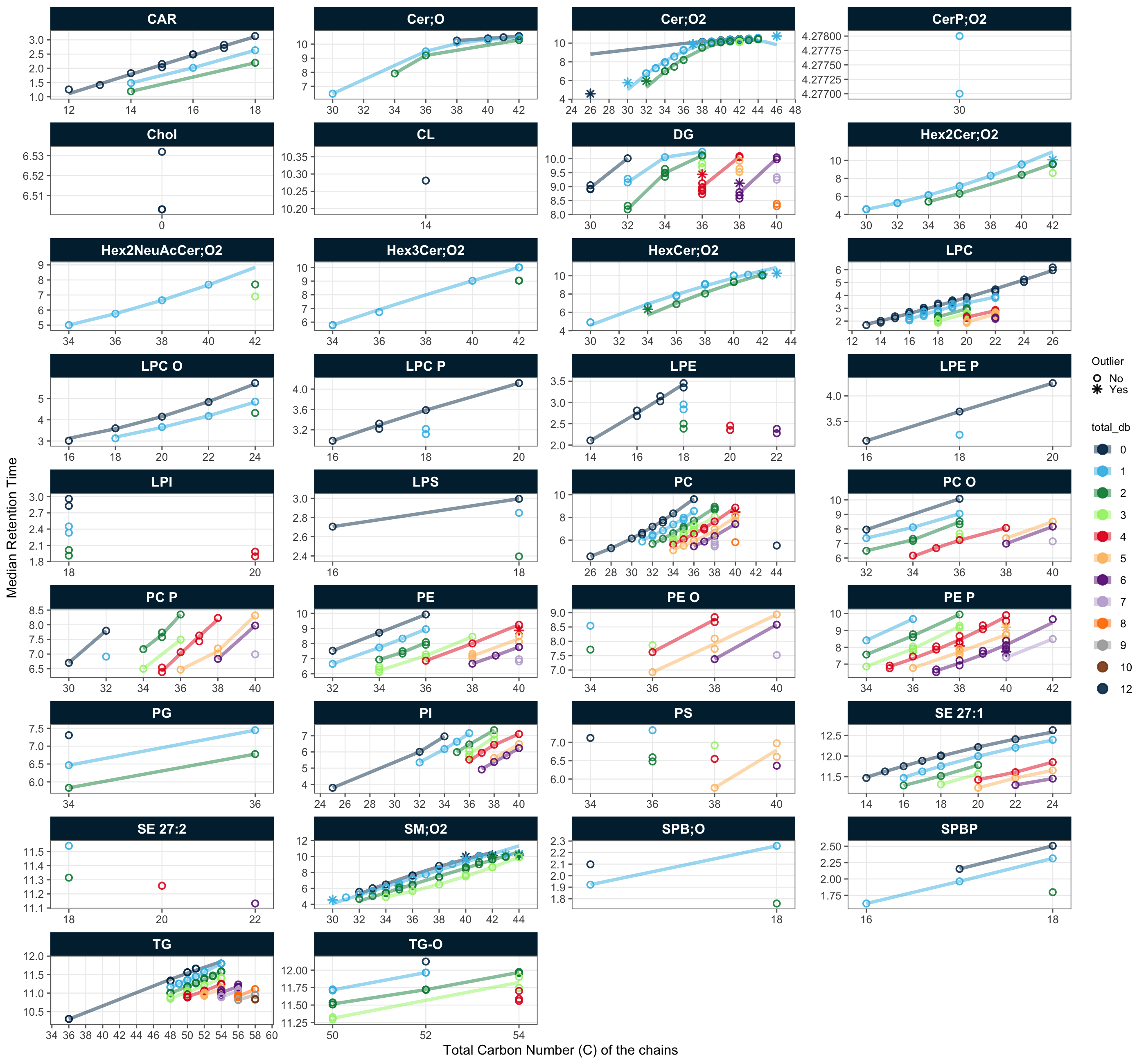
3.4 Feature correlation analysis
Feature correlation analysis was performed as an additional check for potential peak annotation errors. In this analysis, feature pairs exhibiting high correlation (Pearson’s r > 0.98), based on their raw peak areas, were visualized using scatter plots.
# this below is to exclude a sample that has a very low intensity for all features, see next steps for
# details
plot_feature_correlations(
  mexp,
  variable = "intensity",
  qc_types = c("SPL", "BQC", "TQC"),
  point_size = 0.5, cor_min = 0.98, point_stroke = 0.1, sort_by_corr = TRUE,
  return_plots = TRUE, show_progress = FALSE, log_scale = TRUE,
  cols_page = 5, rows_page = 6, font_base_size = 5)
ℹ Generating plots (1 page)...#> [[1]]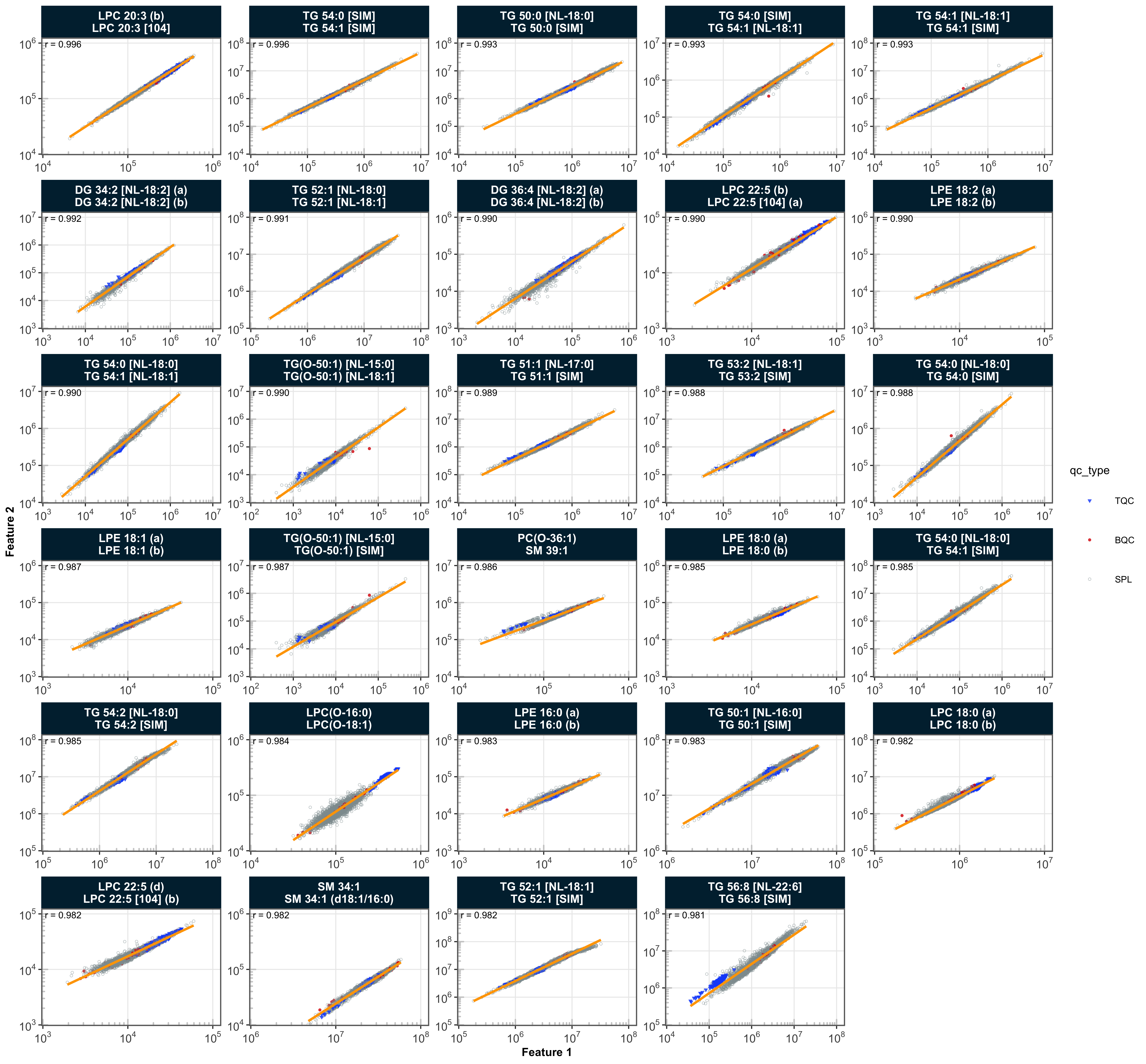
A high correlation (r = 0.986) was observed between features from unrelated classes, namely SM 39:1 and PC O-36:1. As such a strong correlation between unrelated species is highly improbable, this was presumed to be a likely technical or data annotation artefact. Investigation revealed that these features had overlapping retention times, and the M+1 isotope of SM 39:1 shared the same transition as PC O-36:1. A retention time analysis, confirmed with the previously mentioned online resource, indicated that PC O-36:1 should elute after SM 39:1. However, the peak corresponding to PC O-36:1 was found at the end of the MRM window and was partially truncated, which likely contributed to a peak picking error. Due to this truncation of the PC O-36:1 peak, this feature was excluded from subsequent analysis.
mexp <- exclude_features(
  mexp,
  features = "PC(O-36:1)", clear_existing = TRUE)
✔ 1 feature was excluded for downstream processing. Please reprocess data.3.5 Summing up LysoPL and DG isomers
Highly correlating feature pairs from above analysis were found to consist of numerous lysophospholipid (lyso-PL) sn-1/sn-2 isomers and diacylglycerol (DG) isomer peaks. This is an expected observation, as spontaneous positional isomerization, or acyl migration, is known to occur in vitro during sample preparation and storage (Okudaira et al. 2014). Therefore, lyso-PL and DG isomer pairs were summed into a single feature before subsequent processing.
mexp <- data_sum_features(mexp)3.6 PCA to check for potential technical outliers
To obtain an overview of the data and to perform an additional check for potential outlier samples, a Principal Component Analysis (PCA) was conducted based on the raw peak areas of all detected features. The results show that the BQC samples cluster within the study samples, whereas the TQC samples form a distinct group. Closer inspection reveals that TQCs from the last four batches are separated from the other TQCs. Many samples from these same batches are also found in the lower-left area of the plot, outside the bulk of the sample points. Furthermore, BQCs located outside of the main BQC cluster were observed, which are primarily from batches P-30 to P-38.
plot_pca(
  data = mexp,
  variable = "intensity",
  filter_data = FALSE,
  pca_dims = c(1, 2), labels_threshold_mad = 5,
  labels_column = "analysis_order",
  qc_types = c("BQC", "TQC", "LTR", "NIST", "SPL"),
  ellipse_variable = "qc_type",
  log_transform = TRUE, shared_labeltext_hide = "_MS-5", point_size = 0.7,
  point_alpha = 0.7, font_base_size = 8, ellipse_alpha = 0.3,
  include_istd = FALSE,
  show_labels = TRUE, label_font_size = 1.5,
  legend_position = "right", legend_size = 0.7)
! 66 features contained missing or non-numeric values and were exluded.✔ The PCA was calculated based on `feature_intensity` values of 741 features.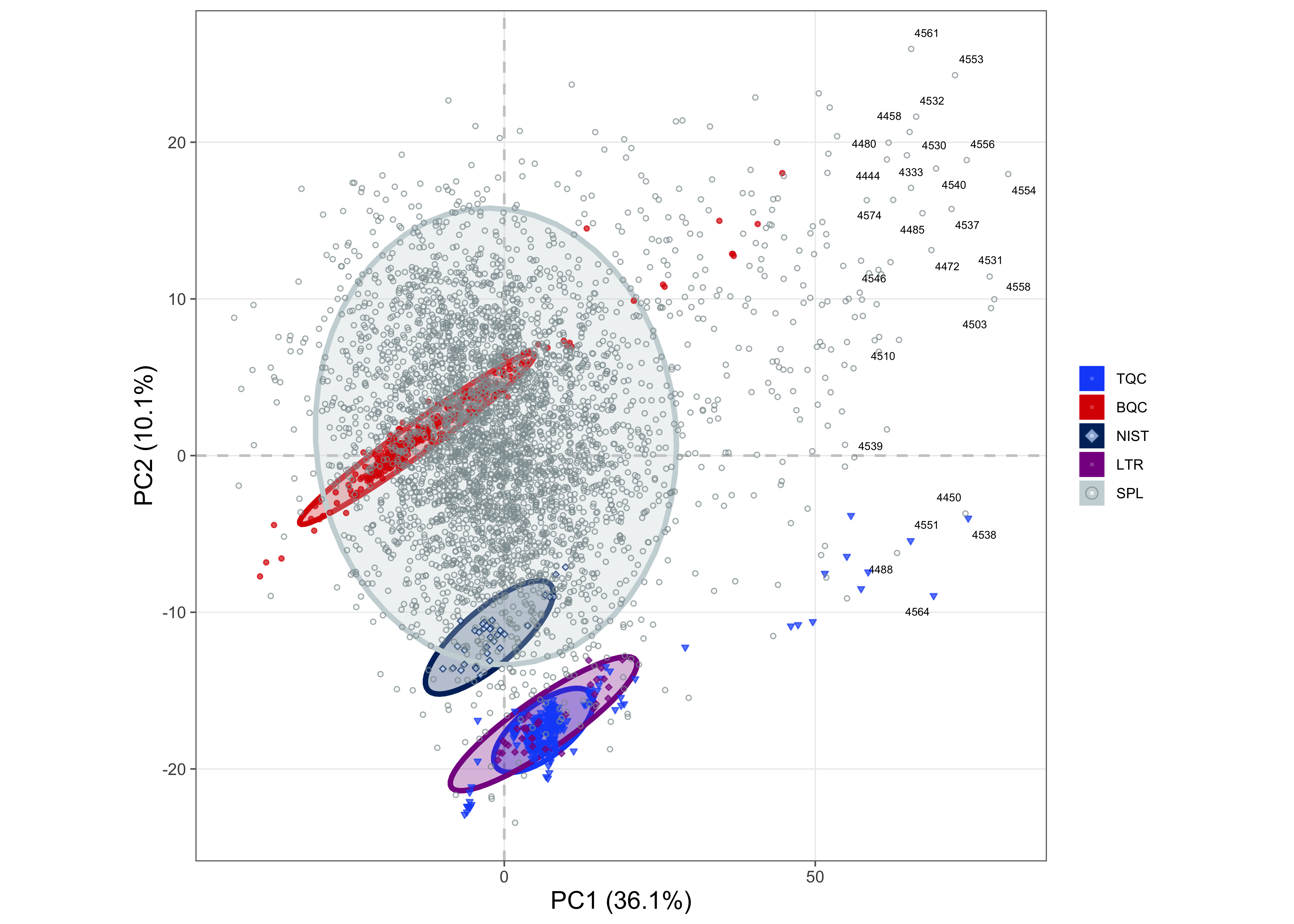
The loadings of the principal components (PC) revealed which features contribute to the variability in the data. While PC1 was contributed to by many features at similar levels, PC2 showed high loadings for numerous lyso-PC species. This may indicate systematic effects during sample preparation and/or analysis that specifically affected this class of lipids.
plot_pca_loading(
  data = mexp,
  variable = "feature_intensity",
  include_istd = FALSE,
  pca_dims = c(1, 2, 3, 4), top_n = 70, font_base_size = 7,
  #qc_types = c("SPL", "BQC", "TQC", "LTR"),
  log_transform = TRUE,
  #point_size = 1, point_alpha = 0.7, font_base_size = 8, ellipse_alpha = 0.3,
  #include_istd = FALSE,
  #show_labels = TRUE,label_font_size = 2,
  #shared_labeltext_hide = NA
) +
  theme(
    plot.title = element_blank(),
    legend.position = "inside", legend.direction = "vertical",
    legend.text = element_text(size = 8 * 0.7),
    legend.title = element_text(size = 8 * 0.7),
    legend.key.size = unit(6 * 0.7, "pt"),
    legend.position.inside = c(0.96, 0.06))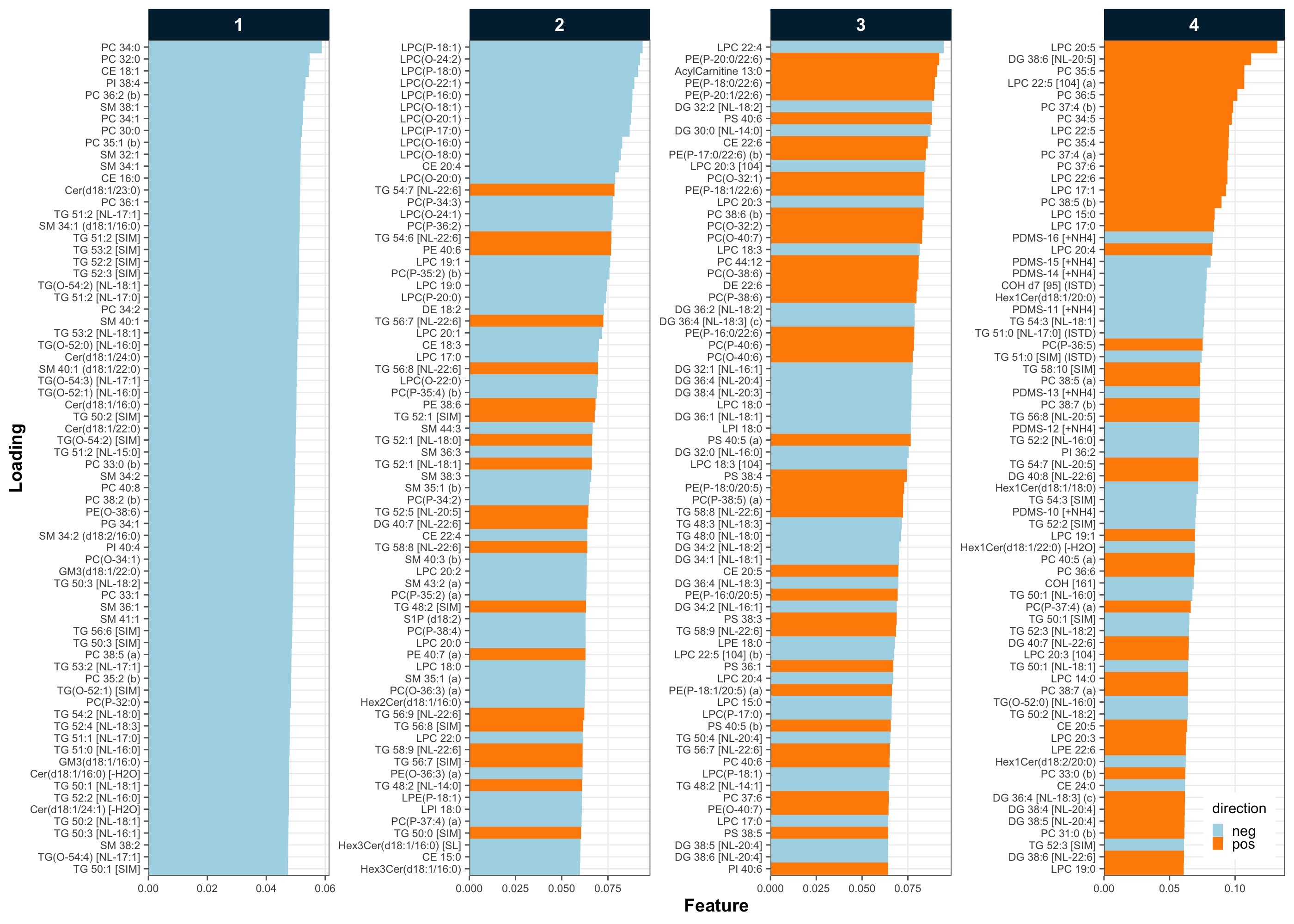
3.7 Matrix effects
To assess potential matrix effects arising from differences between individual samples, the signal distributions of the internal standards (ISTDs) were plotted for each sample type. The signals correspond to the median of batch-wise normalized signals. Cholesterol and the triglyceride (TG) ISTDs exhibited considerably higher matrix effects relative to other ISTDs, as indicated by the wider distributions of their normalized intensities. On average, the Technical QC (TQC) samples displayed lower ISTD signals compared to the Batch QC (BQC) and study samples.
plot_matrixeffects(
  mexp,
  variable = "intensity",
  batchwise_normalization = TRUE, only_istd = FALSE,
  include_qualifier = FALSE,
  include_feature_filter = "ISTD",
  exclude_feature_filter = "95|CL|25|d17\\:0|C1P|H2O",
  y_lim = c(50, 150), point_alpha = 0.05, box_alpha = 0.3, point_size = 0.2,
  box_linewidth = 0.2, font_base_size = 7, min_median_value = 1000)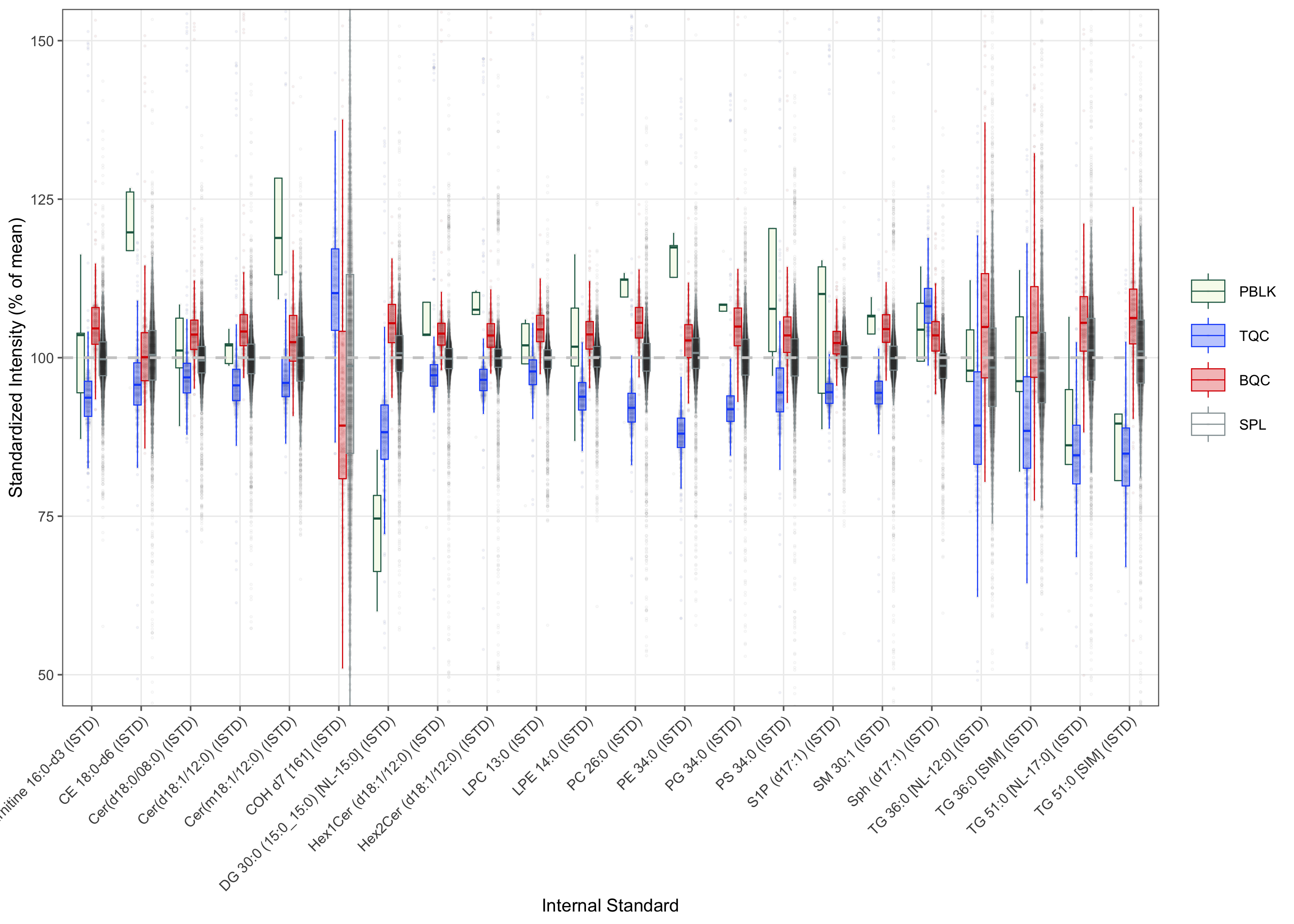
3.8 Isotope correction
The measured, fully saturated phosphatidylcholine (PC) species, i.e., PC 26:0 (ISTD), PC 28:0, PC 30:0, PC 32:0, PC 34:0, and PC 36:0, coelute with the sphingomyelin (SM) species SM 30:1 (ISTD), SM 32:1, SM 34:1, SM 36:1, SM 38:1, and SM 40:1, respectively. Since the M+3 isotopes of these SM species share the same transition as the corresponding PC species, this can lead to an overestimation of PC concentrations. Therefore, an isotope correction was applied to these PC species based on the relative abundance of the SM M+3 isotopes. The correction factors, provided via the feature metadata, were derived using the LICAR method (Gao et al. 2021).
The corresponding QC plot shows that relevant interference is present for PC 26:0 (ISTD), PC 28:0, and PC 30:0, and that PC 36:0 in particular had interference of up to 50%. In the case of PC 36:0, the interference contributed an average of 20% to the signal, ranging from 50% to negative values after correction. Instances where the correction was greater than the PC 36:0 peak area may be a result of analytical variability in both features or the presence of other interferences not accounted for in the SM 40:1 species. Any downstream analysis results for PC 36:0 must be interpreted with consideration of this substantial correction.
mexp <- correct_custom_interferences(mexp)! Interference correction led to 271 negative or zero values in 2 features (samples/QCs). Please verify the correction, or set `neg_to_na = TRUE`.! 1 feature(s) became strongly negative (below -25% of raw) after correction: "PC 36:0". This may indicate a mis-defined interference or an unmodeled effect; please verify.! 1 corrected feature(s) are internal standards: "PC 26:0 (ISTD)". Correcting an ISTD shifts the normalization of every feature it standardizes; please verify.✔ Interference correction applied to 6 of 767 feature(s) (0 isotopic, 6 custom edge(s)).plot_interference_correction(
mexp,
y_lim = c(-10, 110),
qc_types = c("LTR", "NIST", "SPL", "TQC", "BQC"))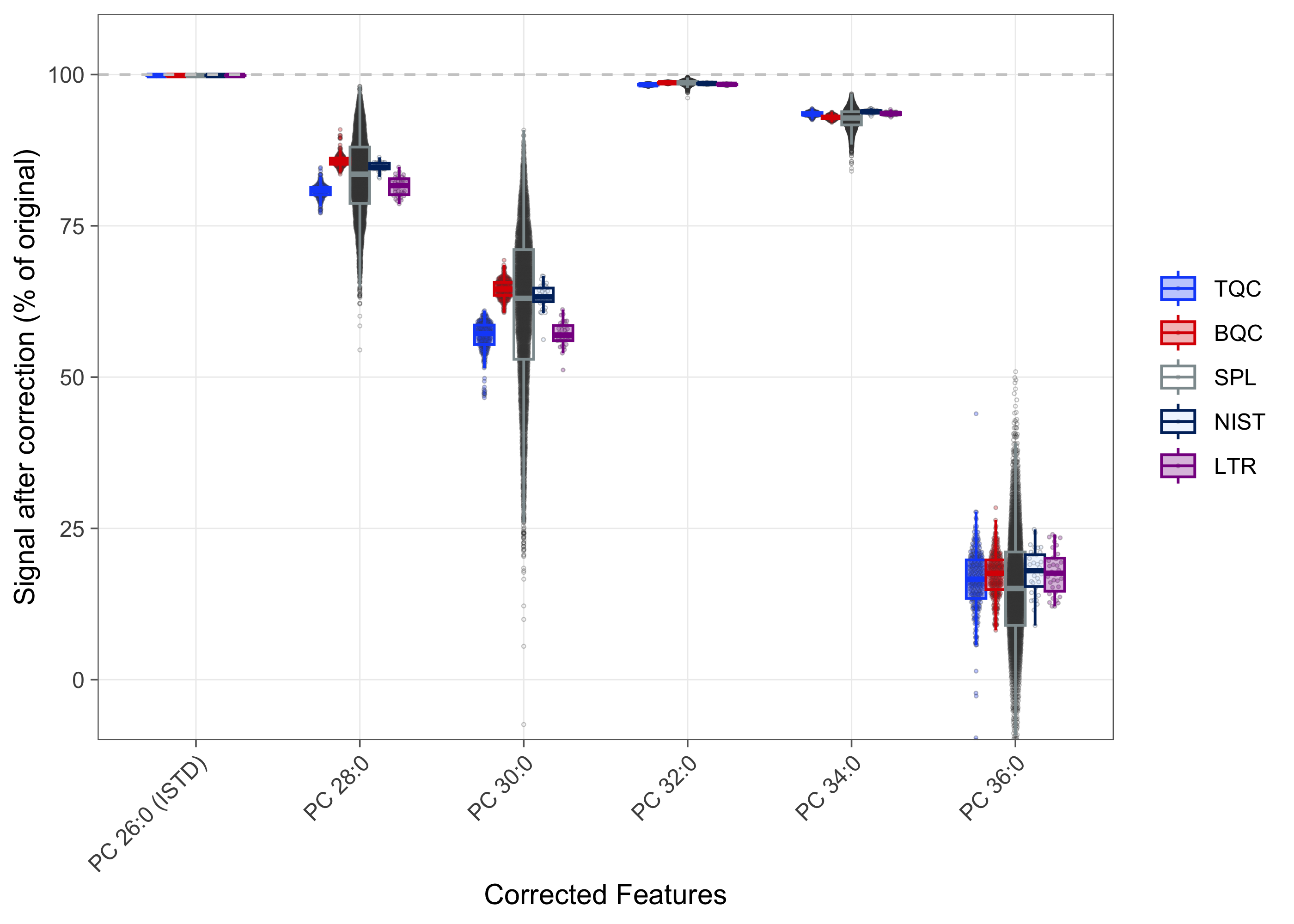
3.9 Normalization and Quantification
The raw intensities were first normalized by their corresponding ISTD, as defined in the feature metadata. Concentrations were then calculated based on the spiked-in ISTD amounts and the sample amounts, which were also defined in the corresponding metadata.
mexp <- normalize_by_istd(mexp, ignore_missing_annotation = FALSE)✔ 713 features normalized with 25 ISTDs in 4494 analyses.mexp <- quantify_by_istd(mexp)✔ 741 feature concentrations calculated based on 26 ISTDs and sample amounts of 4494 analyses.✔ Concentrations are given in μmol/L.The PCA plot of the normalized and quantified data revealed that most TQC samples clustered together. However, the TQCs from batch P-43 formed a distinct cluster in the lower right corner, and TQCs from the last four batches (P-01 to P-04) were also separated from the main TQC cluster. A separate cluster of BQCs, distinct from the main group in the top right corner, was composed primarily of samples from batches P-30 to P-38. These batches also contained BQCs that were identified as outliers in the PCA on raw intensities. This observation suggests that the normalization procedure was insufficient to correct for the observed differences in these BQC samples.
plot_pca(
  data = mexp,
  variable = "conc",
  filter_data = FALSE,
  pca_dims = c(1, 2),
  labels_column = "analysis_order",
  labels_threshold_mad = 4,
  qc_types = c("BQC", "TQC", "LTR", "NIST", "SPL"),
  ellipse_variable = "qc_type",
  log_transform = TRUE, point_size = 0.7, point_alpha = 0.7,
  font_base_size = 8, ellipse_alpha = 0.3,
  include_istd = FALSE,
  show_labels = TRUE, label_font_size = 1.5)
! 68 features contained missing or non-numeric values and were exluded.✔ The PCA was calculated based on `feature_conc` values of 741 features.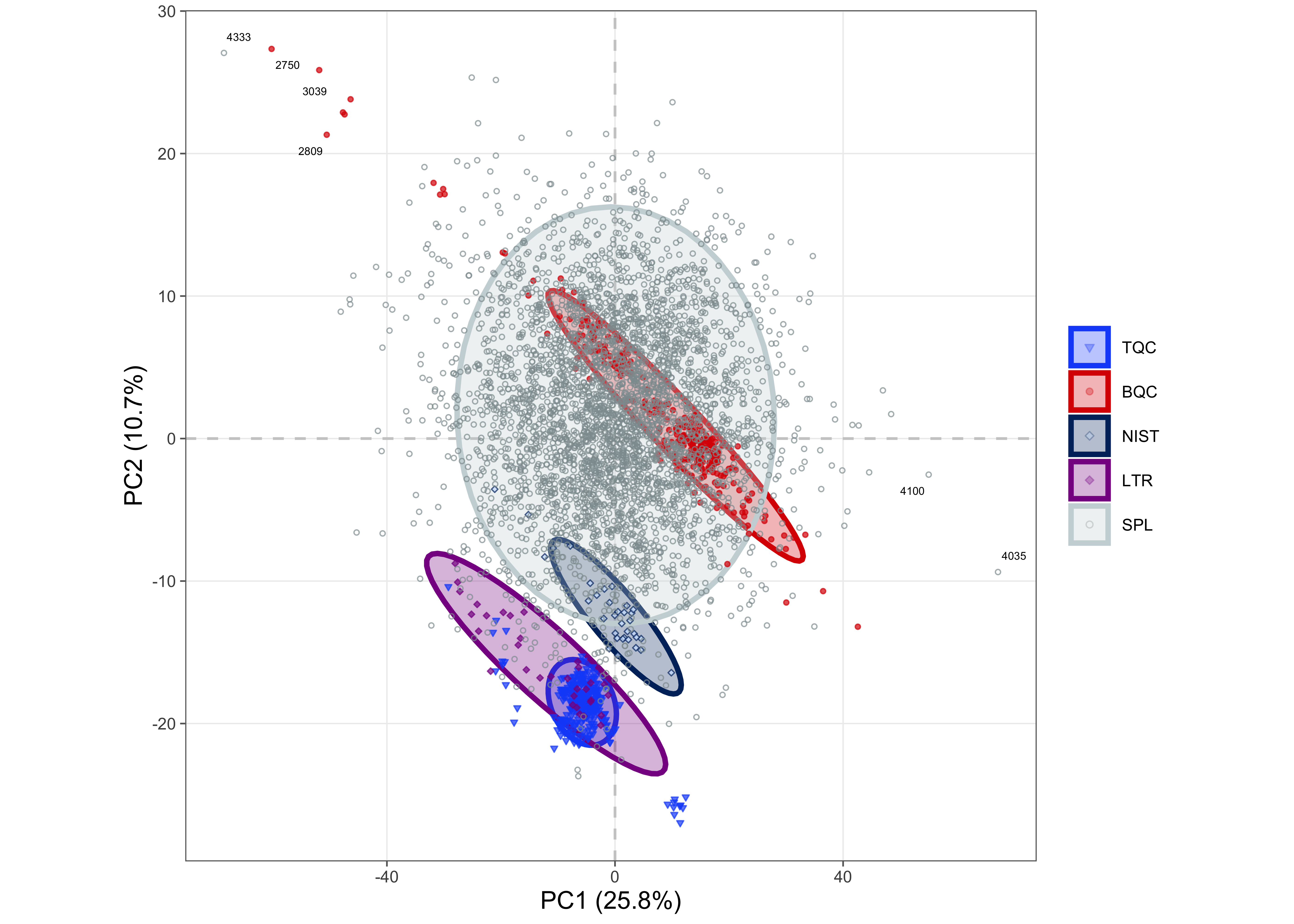
3.10 Removal of batches with identified technical issues
Based on the RunScatter plots and the PCA of the concentrations, it became apparent that batches P-42 and P-43 exhibited technical issues. These batches, which consisted of re-run samples from previous batches, had problems that were not fully resolved by ISTD normalization. Therefore, these batches were excluded from further analysis.
ids_reruns <- mexp@annot_analyses |>
  filter(batch_id %in% c("P-43", "P-42")) |>
  pull(analysis_id)

# The dataset and annotation tables are filtered directly here, as
# exclude_analyses() at this point would require re-processing the data
mexp@dataset <- mexp@dataset |> filter(!analysis_id %in% ids_reruns)
mexp@annot_analyses <- mexp@annot_analyses |>
  filter(!analysis_id %in% ids_reruns)
mexp@annot_responsecurves <- mexp@annot_responsecurves |>
  filter(!analysis_id %in% ids_reruns)
3.11 Inspection of individual features concentrations across the run order
The calculated concentrations of individual features were plotted against the analysis order using RunScatter plots. In the examples shown below, some features did not show any marked drift or batch effects (e.g. SM 34:1). In contrast, clear drift effects within batches were visible for lyso-PC features, while other features exhibited batch effects (e.g., PC 36:4) or drifts that spanned across multiple batches (e.g., PI 38:4). The presence of these drift and batch effects indicates that ISTD normalization was insufficient to correct for such analytical artifacts. Therefore, further data correction is required to minimize these effects, as described in the next section.
plot_runscatter(
  mexp,
  variable = "conc",
  filter_data = FALSE,
  qc_types = c("SPL", "BQC", "TQC", "LTR"),
  include_feature_filter = paste0(
    "PC 34\\:2|PC 36\\:4|PE 38\\:4|PI 38\\:4|PC 38\\:6|CE 18\\:1|",
    "Cer d18\\:1\\/16\\:0|TG 52\\:3|SM 34\\:1|TG 56\\:3|LPC 18\\:1"),
  #y_min = 0.00,
  #y_max = 0.15,
  #plot_range = c(0, 910),
  show_reference_lines = TRUE,
  ref_qc_types = "SPL",
  reference_fill_color = "#111111", reference_k_sd = 3, point_size = 0.5,
  point_border_width = 0.1, font_base_size = 6, cols_page = 2,
  rows_page = 6, cap_outliers = TRUE, reference_sd_shade = FALSE,
  #batch_zebra_stripe = TRUE,
  output_pdf = FALSE)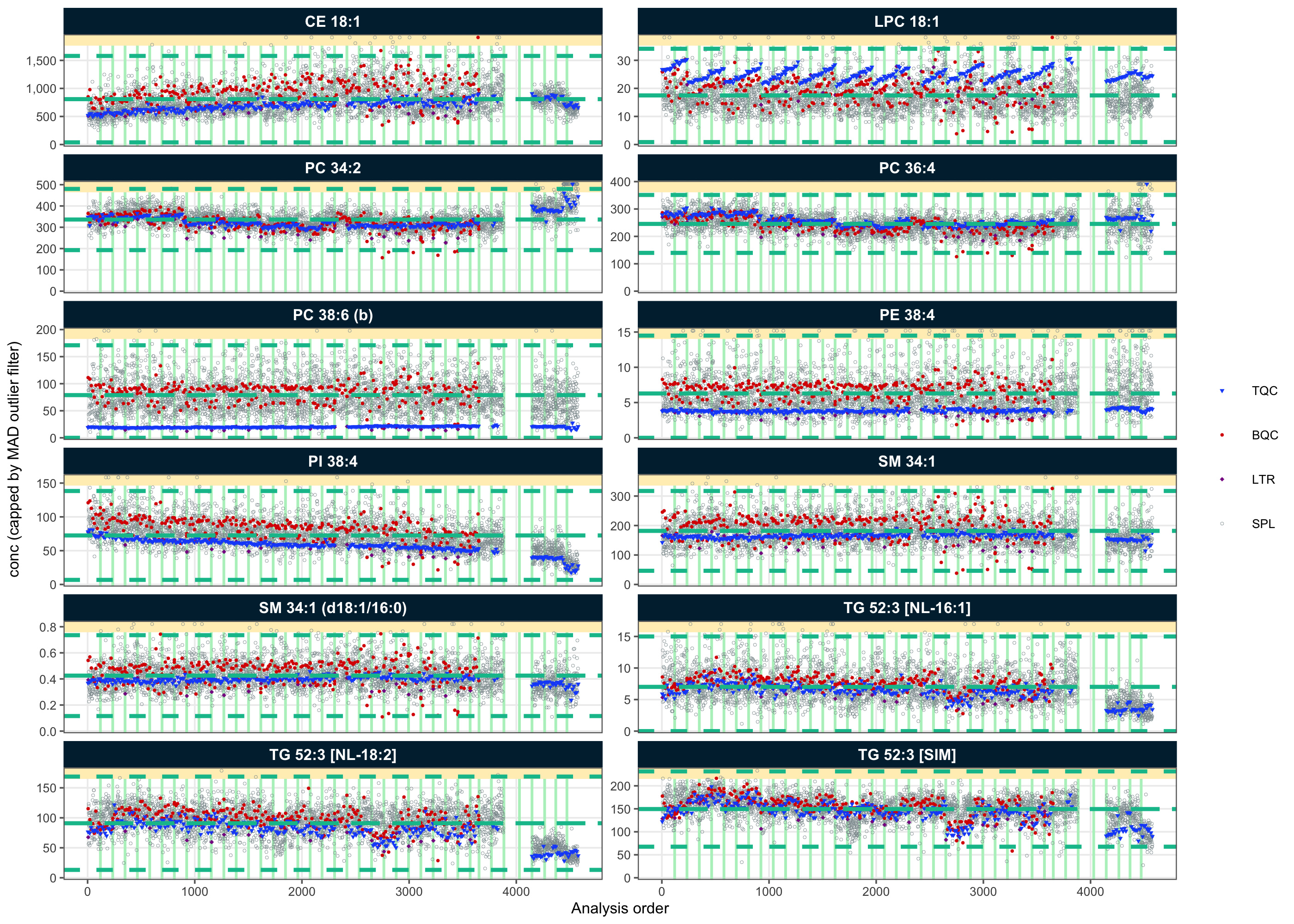
3.12 Drift and Batch Correction
While QC-based drift correction is typically used for such metabolomics and lipidomics datasets, we concluded that the QC samples in this dataset did not adequately represent the drifts observed in the study samples. We therefore opted for a sample-based Gaussian Kernel smoothing approach, assuming that the samples had been fully stratified and randomized. kernel_size sets the number of neighbouring samples over which the trend is smoothed, and outlier_ksd excludes points lying more than that many standard deviations from the local trend so that individual outliers do not distort it. After the within-batch smoothing, the batches were re-aligned using sample-based median centering.
mexp <- correct_drift_gaussiankernel(
  mexp,
  variable = "conc",
  ref_qc_types = "SPL",
  batch_wise = TRUE, kernel_size = 10, outlier_filter = TRUE,
  outlier_ksd = 5, recalc_trend_after = TRUE, show_progress = FALSE)
! 34 feature(s) contain one or more zero or negative `conc` values. Verify your data or use `log_transform_internal = FALSE`.! 28 features showed no variation in the study sample's original values across analyses. ! 28 features have invalid values after smoothing. NA will be be returned for all values of these faetures. Set `use_original_if_fail = FALSE to return orginal values..! Smoothing failed for 28 feature(s) in all batches. Please check data, metadata, and fit parameters.! Smoothing failed for 28 feature(s) in at least one batch: C1P (d18:1/16:0), C1P (d18:1/16:0) [-H2O], C1P (d18:1/26:0), C1P (d18:1/26:0).... Please check data, metadata and fit parameters.✔ Drift correction was applied to 713 of 741 features (batch-wise).ℹ The median per-feature CV change of all features in study samples was -1.42% (range: -15.44% to 4.47%; a positive value means the CV increased). The median CV across all features across batches decreased from 43.53% to 42.25%.
mexp <- correct_batch_centering(
  mexp,
  ref_qc_types = "SPL",
  variable = "conc")
! Adding batch correction on top of `conc` drift-correction.✔ Batch median-centering of 38 batches was applied to drift-corrected concentrations of all 767 features.ℹ The median per-feature CV change of all features in study samples was -1.09% (range: -37.50% to 79.10%; a positive value means the CV increased). The median CV across all features decreased from 43.94% to 42.31%.After applying the drift and batch correction, the RunScatter plots for the same features showed that the drift and batch effects observed in the study samples were minimized. However, because these corrections were based on the study samples, drift and batch effects appear to have been introduced into the QC samples. This further indicates that the QC samples did not adequately represent the analytical variations affecting the study samples.
plot_runscatter(
  mexp,
  variable = "conc",
  filter_data = FALSE,
  #include_feature_filter = "ISTD",
  qc_types = c("SPL", "BQC", "TQC", "LTR"),
  include_feature_filter = paste0(
    "PC 34\\:2|PC 36\\:4|PE 38\\:4|PI 38\\:4|PC 38\\:6|CE 18\\:1|",
    "Cer d18\\:1\\/16\\:0|TG 52\\:3|SM 34\\:1|TG 56\\:3|LPC 18\\:1"),
  #y_min = 0.00,
  #y_max = 0.15,
  #plot_range = c(0, 910),
  show_reference_lines = TRUE,
  ref_qc_types = "SPL",
  reference_fill_color = "#111111", reference_k_sd = 3, point_size = 0.5,
  point_border_width = 0.1, font_base_size = 6, cols_page = 2,
  rows_page = 6, cap_outliers = TRUE, reference_sd_shade = FALSE,
  #batch_zebra_stripe = TRUE,
  output_pdf = FALSE)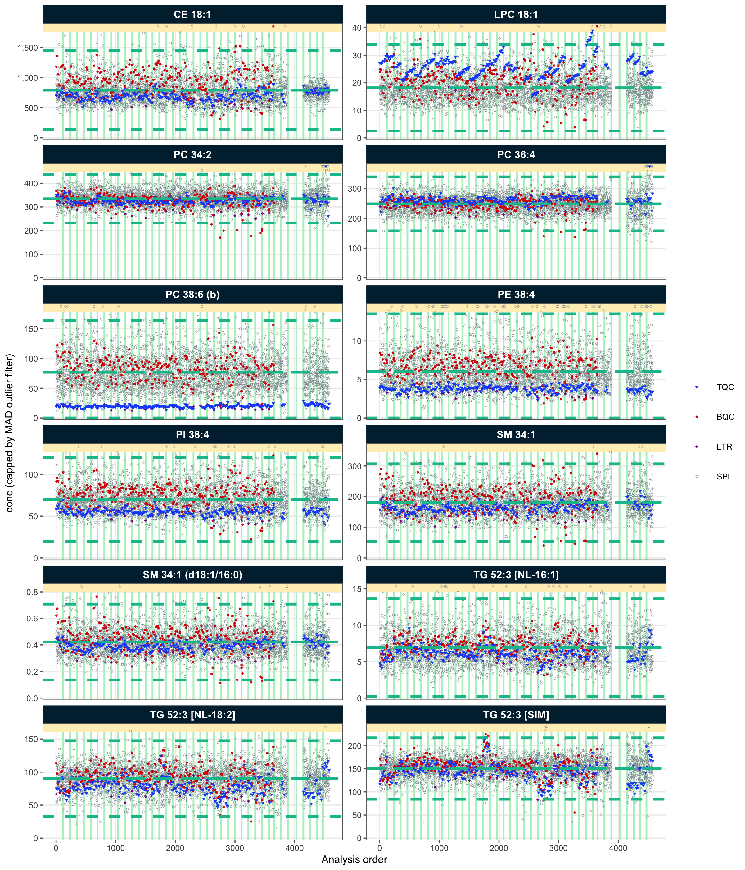
3.13 RunScatter plots of final concentrations of all features
The code below generates PDF files with RunScatter plots for all features, showing the final concentrations after drift and batch correction. Run this code manually if you wish to generate these plots.
plot_runscatter(
  mexp,
  variable = "conc_raw",
  #include_feature_filter = "ISTD",
  qc_types = c("SPL", "BQC", "TQC", "LTR"),
  #include_feature_filter = example_species,
  #y_min = 0.00,
  #y_max = 0.9,
  #plot_range = c(0, 910),
  show_reference_lines = TRUE,
  ref_qc_types = "SPL",
  reference_fill_color = "#111111", reference_k_sd = 3, show_trend = TRUE,
  point_size = 1, font_base_size = 6, cols_page = 2, rows_page = 3,
  cap_outliers = FALSE, reference_sd_shade = FALSE, show_progress = FALSE,
  #batch_zebra_stripe = TRUE,
  multithreading = FALSE, # set TRUE (needs mirai, carrier, qpdf) to parallelise PDF export across mirai daemons
  output_pdf = TRUE,
  path = "./output/Dataset3_runscatter_rawConc_all.pdf")

plot_runscatter(
  mexp,
  variable = "conc",
  #include_feature_filter = "ISTD",
  qc_types = c("SPL", "BQC", "TQC", "LTR"),
  #include_feature_filter = example_species,
  #y_min = 0.00,
  #y_max = 0.9,
  #plot_range = c(0, 910),
  show_reference_lines = TRUE,
  ref_qc_types = "SPL",
  reference_fill_color = "#111111", reference_k_sd = 3, show_trend = TRUE,
  point_size = 1, font_base_size = 6, cols_page = 2, rows_page = 3,
  cap_outliers = FALSE, show_progress = FALSE, reference_sd_shade = FALSE,
  #batch_zebra_stripe = TRUE,
  multithreading = FALSE, # set TRUE (needs mirai, carrier, qpdf) to parallelise PDF export across mirai daemons
  output_pdf = TRUE,
  path = "./output/Dataset3_runscatter_FinalConc_all.pdf")
3.14 QC of normalization and drift/batch correction
Normalization with ISTDs, particularly the non-authentic, class-wide ISTDs used in this analysis, can introduce artifacts that can lead to an increase in sample variability rather than the expected reduction. Similarly, batch and drift correction can introduce artifacts and increase, rather than decrease, analytical variability. The following plot compares the variability of QC and study samples before (raw areas) and after normalization and drift/batch correction (final concentrations). The plot shows that for most QC types and study samples, variability was reduced after normalization and correction, indicating an overall benefit of these processing steps. However, while the study samples exhibited decreased CVs after processing, the BQC and TQC samples showed increases. This may be another illustration that the QC samples did not fully represent the analytical variations affecting the study samples.
mexp <- calc_qc_metrics(
  mexp,
  use_robust_cv = FALSE, use_batch_medians = TRUE)
! %CV not computed for 141888 feature×QC-type×variable combinations with fewer than 3 replicates (LTR: 70937, NIST: 70936, TQC: 15).✔ QC metrics calculated for 767 features across 8 sample types, including normalized-intensity, concentration, and response-curve statistics.plot_normalization_qc(
plot_type = "diff",
data = mexp,
before_norm_var = "intensity",
after_norm_var = "conc",
y_lim = c(-15, 15), x_lim = c(0, 75),
qc_types = c("TQC", "BQC", "SPL", "NIST"),
cols_page = 5, font_base_size = 5, point_size = 0.5,
facet_by_class = TRUE,
include_qualifier = FALSE)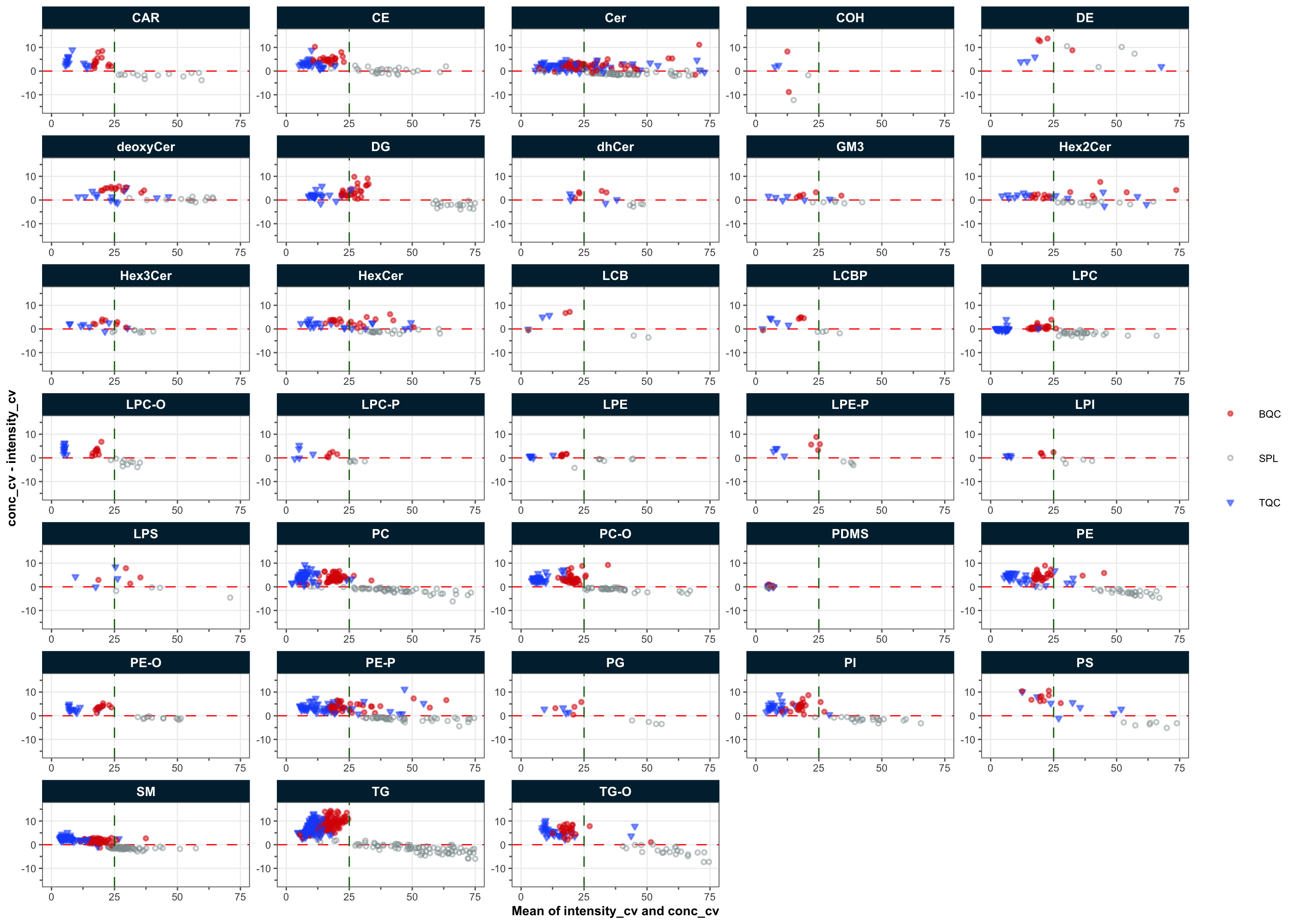
3.15 Process vs instrument variability
To understand how much of the total technical variability comes from the overall process (sample preparation and the instrument variability) or just from the instrument, the CVs of a feature in batch (process) QC samples (a pooled sample repeatedly extracted and measured along with the study samples) and the technical QC samples (a pooled extract measured at regular intervals) are compared (Broadhurst et al. 2018). The plot below shows that for most features, the variability in the BQCs is higher than in the TQCs, indicating that sample preparation contributes considerably to the overall technical variability.
mrmhub::plot_qcmetrics_comparison(
  mexp,
  plot_type = "diff",
  y_shared = TRUE,
  x_variable = "conc_cv_tqc",
  y_variable = "conc_cv_bqc",
  log_scale = FALSE, equality_line = TRUE,
  facet_by_class = TRUE,
  point_size = 2, font_base_size = 5, x_lim = c(0, 25), y_lim = c(-15, 15))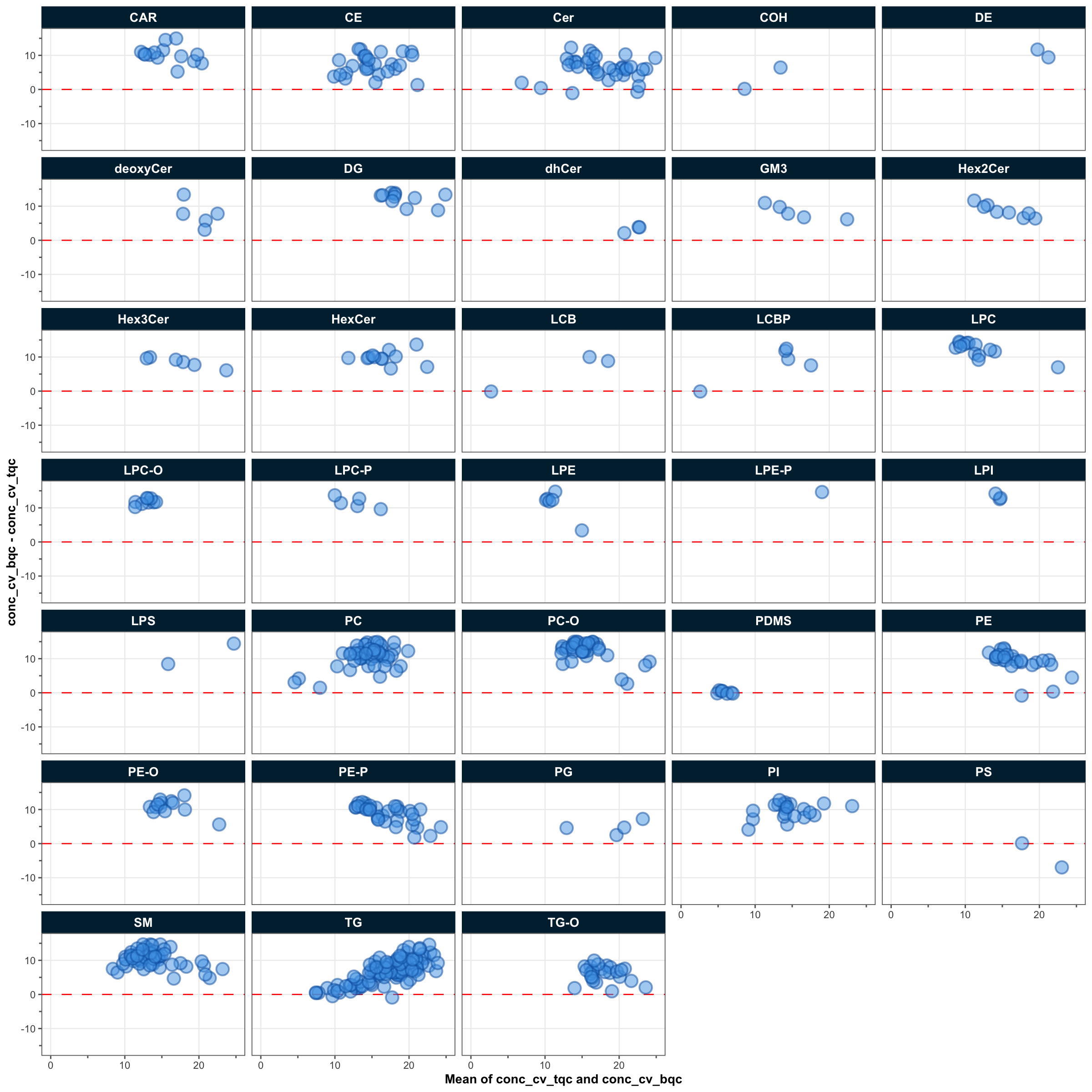
3.16 Effect of feature intensity on technical variability
An analysis of the relationship between feature abundance and technical variability can be used to determine the intensity threshold at which feature signals exhibit increased noise and variance. This information can then be applied during peak picking to set appropriate intensity thresholds for feature detection and to reduce the processing time spent on integrating low-abundance features.
mrmhub::plot_qcmetrics_comparison(
  mexp,
  plot_type = "scatter",
  y_shared = FALSE,
  x_variable = "intensity_median_bqc",
  y_variable = "intensity_cv_bqc",
  log_scale = FALSE, equality_line = FALSE,
  facet_by_class = FALSE,
  point_size = 0.5, font_base_size = 5, x_lim = c(10, Inf),
  y_lim = c(0, 100)) +
  ggplot2::geom_smooth(method = "loess", se = FALSE, span = 0.75) +
  geom_hline(yintercept = 20, linetype = "dashed", color = "grey70") +
  scale_x_log10(
    expand = ggplot2::expansion(mult = c(0, 0.00)),
    breaks = c(1E2, 1E3, 1E4, 1E5, 1E6, 1E7, 1E8)) +
  scale_y_continuous(
    expand = ggplot2::expansion(mult = c(0.03, 0.00)),
    breaks = c(0, 20, 40, 60, 80))
Scale for x is already present.
Adding another scale for x, which will replace the existing scale.
Scale for y is already present.
Adding another scale for y, which will replace the existing scale.
`geom_smooth()` using formula = 'y ~ x'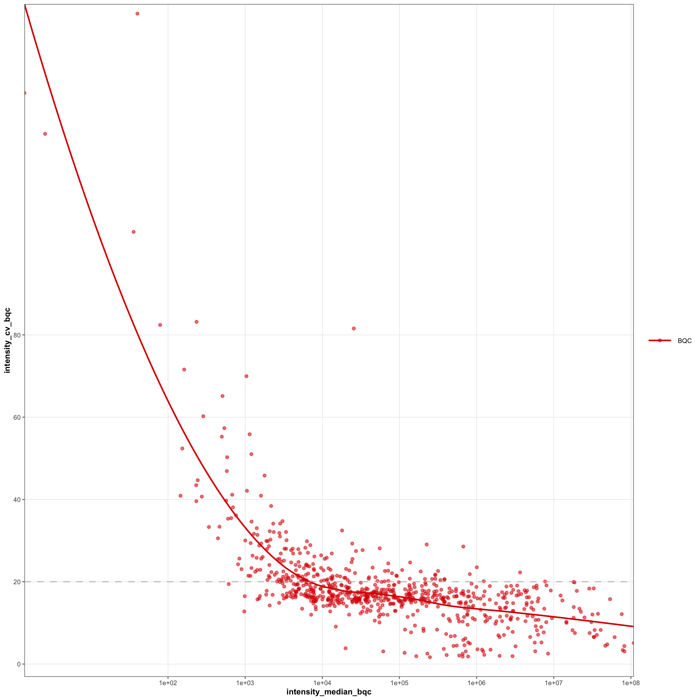
3.17 Response curves
Response curves relate the measured signal to the relative spiked-in amount and are used to assess the linear range and quantitative response of each analyte relative to its internal standard. The examples below show selected analytes together with their ISTDs.
sel_species <- c(
  "PC 26:0 (ISTD)",
  "SM 34:1", "PC 34:2", "CE 18:2", "TG 50:1 [NL-16:0]", "CE 20:4",
  "LPC 18:1")
plot_responsecurves(
  data = mexp,
  variable = "intensity",
  max_regression_value = 100,
  filter_data = FALSE,
  font_base_size = 6, line_width = 0.5, point_size = 1.2,
  include_feature_filter = sel_species,
  output_pdf = FALSE,
  show_progress = FALSE, cols_page = 3, rows_page = 3, return_plots = TRUE,
  legend_position = "inside-br", legend_size = 0.6, show_legend_title = FALSE)[[1]]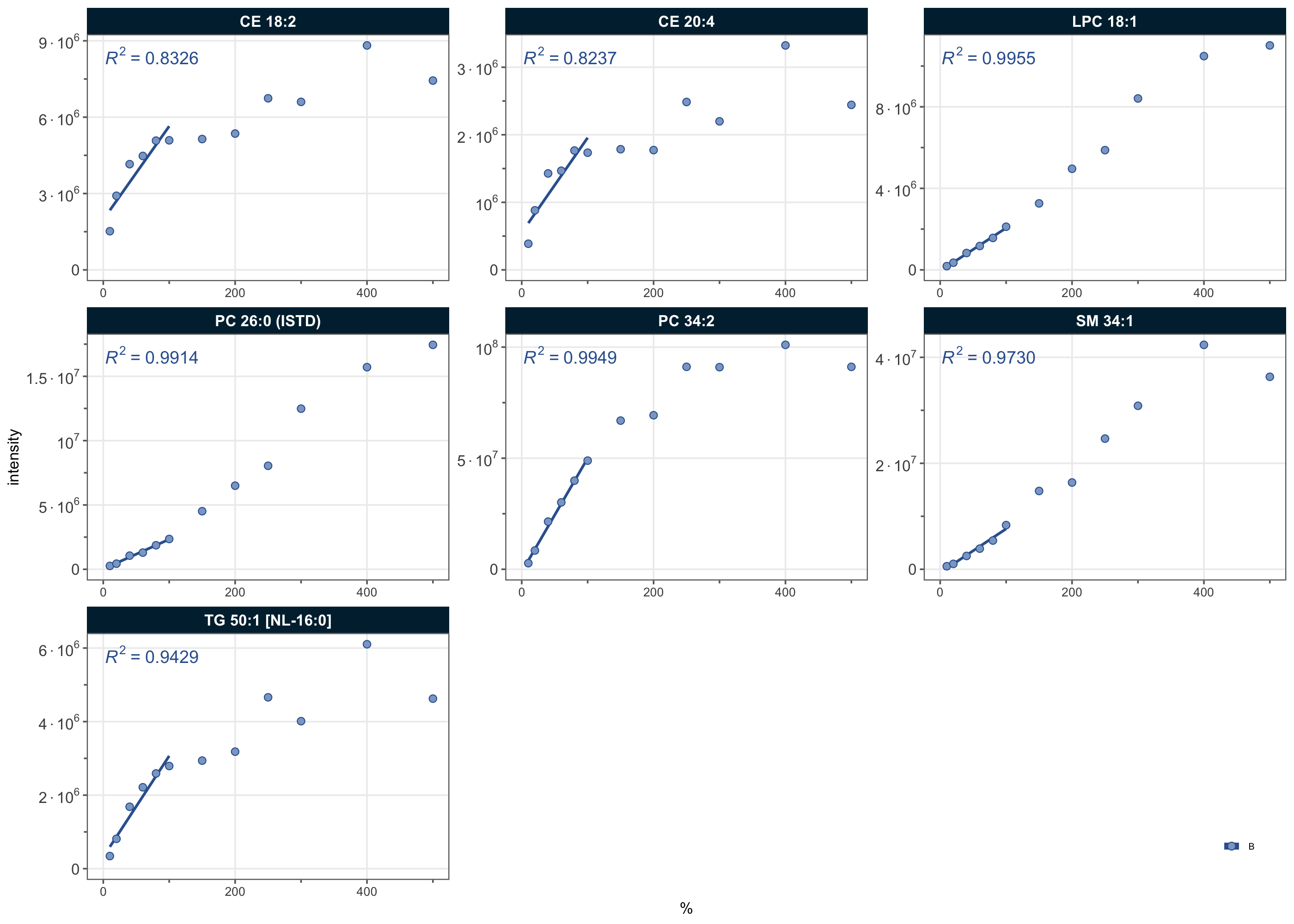
The code below generates PDF files with response curve plots for all features. Run this code manually if you wish to generate these plots.
plot_responsecurves(
  data = mexp,
  variable = "intensity",
  max_regression_value = 100,
  filter_data = FALSE,
  font_base_size = 6, line_width = 0.5, point_size = 1.2, output_pdf = TRUE,
  path = "./output/dataset3-response-curves.pdf",
  show_progress = FALSE, cols_page = 6, rows_page = 5, return_plots = FALSE)
3.18 Feature filter
The QC metrics are recalculated on the corrected concentrations, and the features are then filtered to retain only those meeting the quality criteria for the final dataset. The thresholds combine an adequate response-curve fit (R² ≥ 0.8, slope ≥ 0.5, y-intercept ≤ 0.5), sufficient signal over blank (≥ 10) and absolute intensity (≥ 100), and acceptable precision in the batch QCs (CV ≤ 25 %). A few cholesteryl esters that fail these criteria are retained explicitly via features.to.keep.
mexp <- calc_qc_metrics(
  mexp,
  use_robust_cv = FALSE, use_batch_medians = TRUE,
  include_response_stats = TRUE)
! %CV not computed for 141888 feature×QC-type×variable combinations with fewer than 3 replicates (LTR: 70937, NIST: 70936, TQC: 15).✔ QC metrics calculated for 767 features across 8 sample types, including normalized-intensity, concentration, and response-curve statistics.mexp <- filter_features_qc(
data = mexp,
clear_existing = TRUE, use_batch_medians = TRUE,
include_qualifier = FALSE,
include_istd = FALSE,
response.curves.selection = 1,
response.curves.summary = "mean",
min.rsquare.response = 0.8,
min.slope.response = 0.5,
max.yintercept.response = 0.5,
min.signalblank.median.spl.pblk = 10,
min.intensity.median.spl = 100,
max.cv.conc.bqc = 25,
#max.dratio.sd.conc.bqc = 0.75,
max.prop.missing.conc.spl = 100,
features.to.keep = c(
"CE 20:4",
"CE 22:5", "CE 22:6", "CE 16:0", "CE 18:0"))! The QC parameter min.intensity.median.spl contains NAs for the following features: C1P (d18:1/16:0), C1P (d18:1/16:0) [-H2O], C1P (d18:1/18:0), C1P (d18:1/18:0).... These features failed QC.! The QC parameter min.signalblank.median.spl.pblk contains NAs for the following features: C1P (d18:1/16:0), C1P (d18:1/16:0) [-H2O], C1P (d18:1/18:0), C1P (d18:1/18:0).... These features failed QC.! The QC parameter max.cv.conc.bqc contains NAs for the following features: C1P (d18:1/16:0), C1P (d18:1/16:0) [-H2O], C1P (d18:1/18:0), C1P (d18:1/18:0).... These features failed QC.! The QC parameter max.prop.missing.conc.spl contains NAs for the following features: C1P (d18:1/18:0), C1P (d18:1/18:0) [-H2O], CE 18:1 d7 (ISTD), Cer(d18:0/08:0).... These features failed QC.! The following features were forced to be retained despite not meeting filtering criteria: CE 20:4, and CE 22:5✔
New feature QC filters were defined: 460 of 741 quantifier features meet QC criteria (not including the 26 quantifier ISTD features).3.19 Feature filter Results
The outcome of the filtering is summarized per lipid class, showing how many analytes passed and failed the QC criteria in each class.
# `plot_qc_summary_byclass()` draws one x-axis level per feature class in the QC metrics
# but only summarizes non-ISTD/non-qualifier features. A class made up solely of such
# features is empty in the summary, so the axis has more breaks than labels — which aborts
# the secondary axis under ggplot2 >= 4.0. Drop those phantom classes from a copy first.
mexp_byclass <- mexp
.keep_classes <- mexp@metrics_qc |>
  dplyr::filter(valid_feature, in_data, pass_istd, pass_qualifier) |>
  dplyr::pull(feature_class) |>
  unique()
mexp_byclass@metrics_qc <- dplyr::filter(
  mexp@metrics_qc,
  feature_class %in% .keep_classes)

plot_qc_summary_byclass(
  mexp_byclass,
  font_base_size = 8, legend_position = c(0.77, 0.27), legend_size = 0.7,
  show_legend_title = FALSE)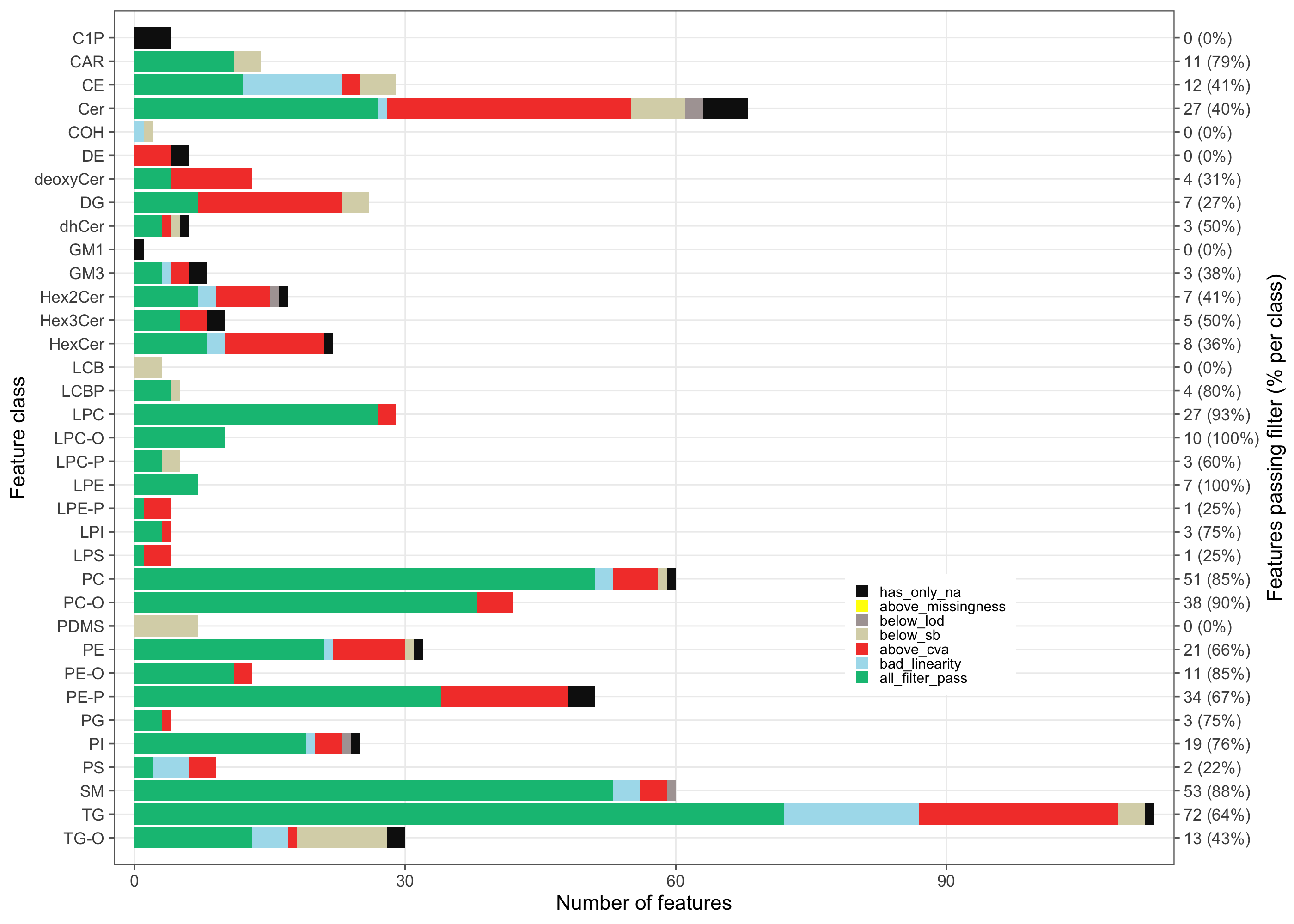
3.20 Feature filter Venn
This plot summarizes the overall filtering outcome, showing how many features passed or failed across all criteria and how the individual QC criteria overlapped in the features they removed.
plot_qc_summary_overall(mexp)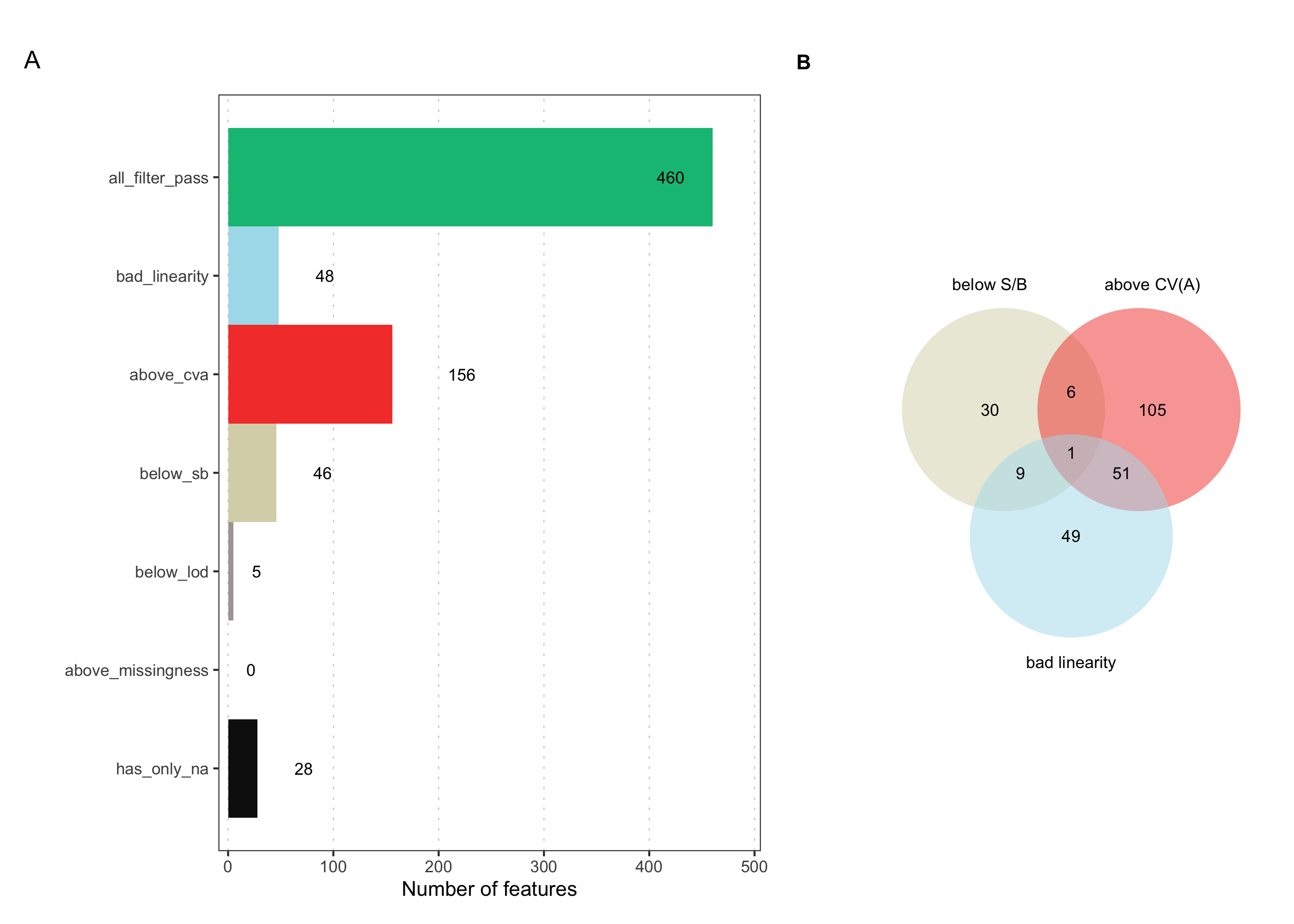
3.21 PCA plots of the final dataset
The PCA plot shows that the overall structure remains similar to that observed before correction. The TQCs are more dispersed than before correction, but still form a relatively compact cluster. In contrast, the BQCs, LTR, and NIST exhibit long elliptical clusters spanning a larger area, indicating systematic variability introduced during sample processing that was not fully corrected by ISTD normalization and drift/batch correction.
plot_pca(
  data = mexp,
  variable = "conc",
  filter_data = TRUE,
  pca_dims = c(1, 2),
  labels_column = "analysis_order",
  labels_threshold_mad = 5,
  qc_types = c("BQC", "TQC", "LTR", "NIST", "SPL"),
  ellipse_variable = "qc_type",
  log_transform = TRUE, point_size = 0.7, point_alpha = 0.7,
  font_base_size = 8, ellipse_alpha = 0.3,
  include_istd = FALSE,
  show_labels = TRUE, label_font_size = 1.5)
! 5 features contained missing or non-numeric values and were exluded.✔ The PCA was calculated based on `feature_conc` values of 460 features.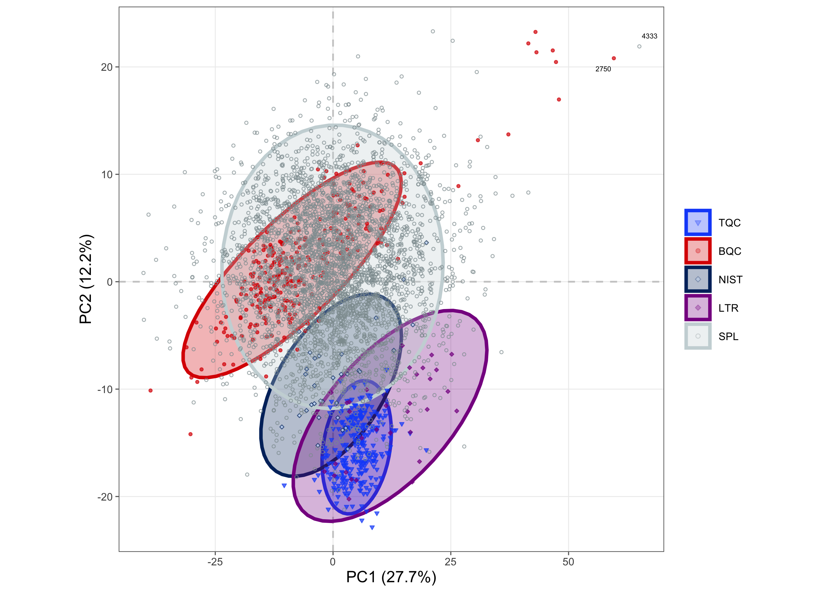
3.22 Lipidome Profile
As a final overview, the feature concentration profile of the filtered dataset is shown below. Validating the concentrations, for example, those of the most abundant species, the summed concentrations per lipid class, or the ratios between lipid classes, against in-house reference values or literature data helps ensure that the quantification is within expected ranges and that no major quantification errors are present.
plot_abundanceprofile(
  data = mexp,
  log_scale = TRUE,
  filter_data = TRUE,
  variable = "conc",
  qc_types = "SPL",
  #x_lim = c(-6, 2),
  x_label = NA,
  feature_map = "lipidomics")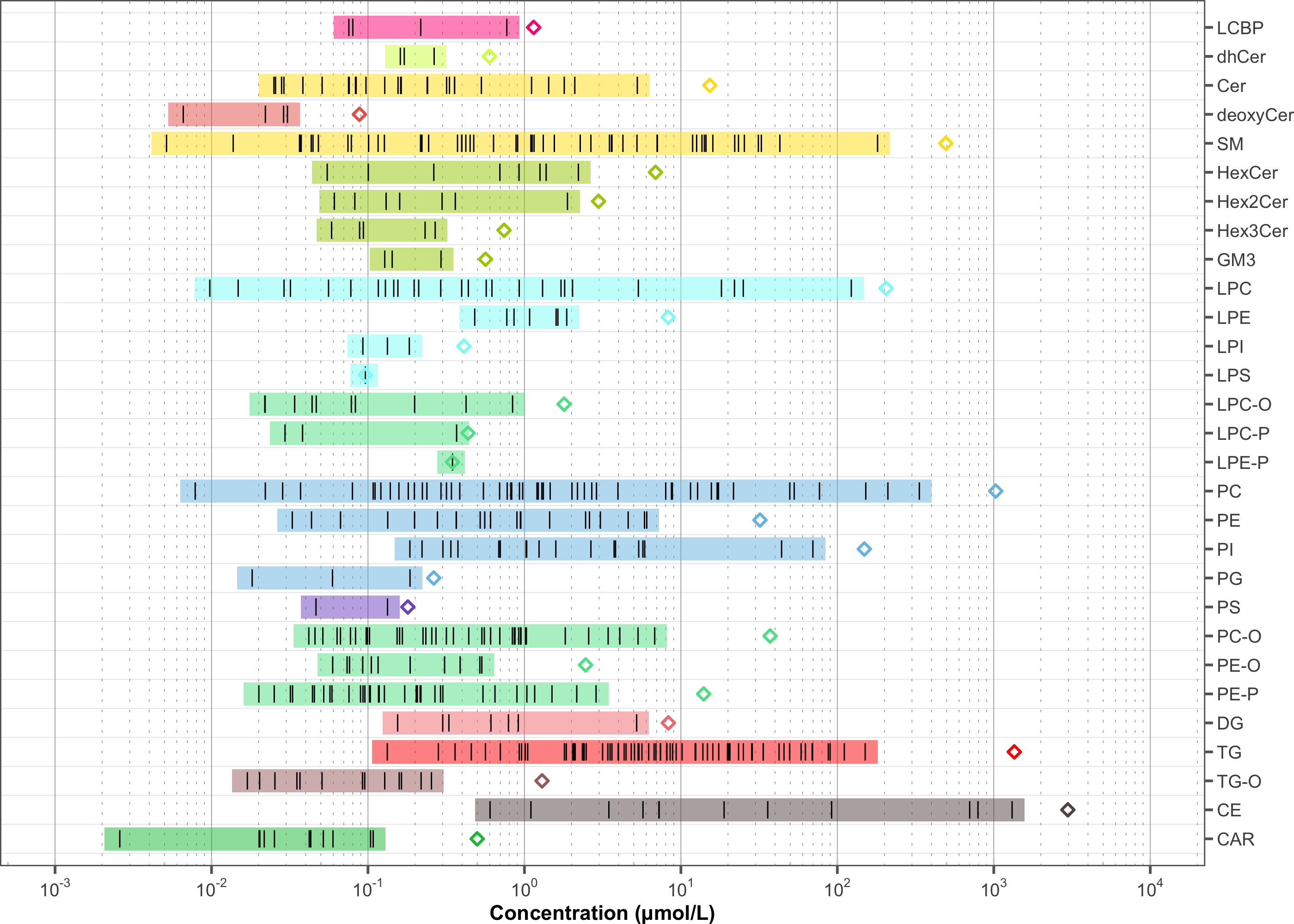
3.23 Export the dataset
The dataset is exported as a CSV file. The user can specify the variable to export, whether to include qualifier features, whether to restrict the output to specific QC types (here the study samples, SPL), and whether to apply the QC feature filter. Two versions are written: all features before the QC filter, and the final dataset restricted to the features that passed it (filter_data = TRUE). Both contain the drift- and batch-corrected concentrations (conc).
save_dataset_csv(
  data = mexp,
  path = "./output/Dataset3_UNFILTERED-feature_conc_uM.csv",
  variable = "conc",
  qc_types = "SPL",
  include_qualifier = FALSE,
  filter_data = FALSE)

save_dataset_csv(
  data = mexp,
  path = "./output/Dataset3_FILTERED-feature_conc_uM.csv",
  variable = "conc",
  qc_types = "SPL",
  include_qualifier = FALSE,
  filter_data = TRUE)
The complete MRMhubExperiment — imported data, metadata and all processing results — is also saved as a single .rds with save_dataset_rds(). This self-contained object can be shared and reopened in any R session with read_dataset_rds(), which verifies an embedded integrity hash, to continue or audit the analysis without re-running the pipeline.
save_dataset_rds(mexp, "./output/Dataset3_mexp.rds")4 References
Broadhurst, David, Royston Goodacre, Stacey N. Reinke, et al. 2018. “Guidelines and Considerations for the Use of System Suitability and Quality Control Samples in Mass Spectrometry Assays Applied in Untargeted Clinical Metabolomic Studies.” Metabolomics 14 (6): 72. https://doi.org/10.1007/s11306-018-1367-3.
Chen, Yuqing, Federico Torta, Hiromi W. L. Koh, et al. 2025. “Metabolomics Profiling in Multi-Ancestral Individuals with Type 2 Diabetes in Singapore Identified Metabolites Associated with Renal Function Decline.” Diabetologia 68 (3): 557–75. https://doi.org/10.1007/s00125-024-06324-z.
De Livera, Alysha M., Daniel A. Dias, David De Souza, et al. 2012. “Normalizing and Integrating Metabolomics Data.” Analytical Chemistry 84 (24): 10768–76. https://doi.org/10.1021/ac302748b.
Gao, Liang, Shanshan Ji, Bo Burla, Markus R. Wenk, Federico Torta, and Amaury Cazenave-Gassiot. 2021. “LICAR: An Application for Isotopic Correction of Targeted Lipidomic Data Acquired with Class-Based Chromatographic Separations Using Multiple Reaction Monitoring.” Analytical Chemistry 93 (6): 31633171. https://doi.org/10.1021/acs.analchem.0c04565.
Huynh, Kevin, Christopher K. Barlow, Kaushala S. Jayawardana, et al. 2019. “High-Throughput Plasma Lipidomics: Detailed Mapping of the Associations with Cardiometabolic Risk Factors.” Cell Chemical Biology 26 (1): 71–84.e4. https://doi.org/10.1016/j.chembiol.2018.10.008.
Livera, Alysha M. De, Marko Sysi-Aho, Laurent Jacob, et al. 2015. “Statistical Methods for Handling Unwanted Variation in Metabolomics Data.” Analytical Chemistry 87 (7): 3606–15. https://doi.org/10.1021/ac502439y.
Okudaira, Michiyo, Asuka Inoue, Akira Shuto, et al. 2014. “Separation and Quantification of 2-Acyl-1-Lysophospholipids and 1-Acyl-2-Lysophospholipids in Biological Samples by LC-MS/MS.” Journal of Lipid Research 55 (10): 2178–92. https://doi.org/10.1194/jlr.D048439.