# Chromatograms are pre-cropped from the INTEGRATOR by_transition PDFs by
# figures/dataset4/dataset4-chromatograms.R and embedded here as static PNGs, so
# the notebook render needs neither the PDFs nor magick/ghostscript.
chrom_dir <- "images/dataset4"
chrom_grob <- function(name) grid::rasterGrob(
png::readPNG(file.path(chrom_dir, paste0(name, ".png"))), interpolate = TRUE)
chrom_gg <- function(name, title, subtitle = NULL) {
ggplot() + annotation_custom(chrom_grob(name)) +
labs(title = title, subtitle = subtitle) +
theme_void(base_size = 8, base_family = "sans") +
theme(plot.title = element_text(size = 8, hjust = 0.5, margin = margin(b = 1)),
plot.subtitle = element_text(size = 6.8, hjust = 0.5, colour = "grey30",
margin = margin(b = 2)))
}
(chrom_gg("integrator_Cortisol", "Cortisol") |
chrom_gg("integrator_Testosterone", "Testosterone"))MRMhub Data Processing Workflow for Dataset 4
Supplementary Code 3
Overview
Dataset 4 is a fully quantitative steroid panel used to validate MRMhub against a vendor pipeline (Agilent MassHunter). Fifteen steroids were measured in human serum with the IBL International Steroid Panel LC-MS kit (cat. 30191875) according to the instructions for use, with modifications. The kit acquires its analytes over two chromatographic panels; only Panel 1 (15 analytes) is used here, which is why every sample identifier carries the _P1 suffix (e.g. Cal A_P1, QC_High1_P1).
Unlike Datasets 1 and 3 (relative lipidomics), this is an externally calibrated absolute assay. The analytical design comprises an external calibration curve (Cal 0–Cal F), low and high quality-control samples (QC_Low1, QC_High1), and external quality-assessment (EQA) samples — SKML ring-trial materials with reference-method-assigned target concentrations (Jansen et al. 2014).
The workflow compares MRMhub and MassHunter at both pipeline stages:
- INTEGRATOR — peak areas from MRMhub-INTEGRATOR vs a MassHunter re-integration of the same raw files (Figure 1).
- QUANT — calibration fits and concentrations, ending in accuracy against the SKML EQA reference values (Figure 2).
Raw Data Processing: Peak Picking and Integration
Raw .d files were converted to mzML and integrated with MRMhub-INTEGRATOR, as described for Datasets 1 and 3. The batch was integrated in two subsets — the system-suitability injections (SST, ten replicate injections) and the assay samples (ASSAY: blanks, calibrators, QCs, EQA samples) — exported as separate long-format tables and combined downstream. INTEGRATOR reports peak areas, retention times and peak metadata in long.csv, and writes per-transition integration plots (the shaded, integrated region) to the by_transition folder.
The same raw files were independently re-integrated in Agilent MassHunter Quantitative Analysis, providing the reference peak areas and concentrations used throughout this document.
The example chromatograms are cropped from the INTEGRATOR by_transition PDFs by figures/dataset4/dataset4-chromatograms.R (run once; requires the magick R package and ghostscript) and embedded here as static images from images/dataset4/. The notebook render itself needs neither.
Data Postprocessing and QC
The postprocessing pipeline is the QUANT module (library(mrmhub)): import the INTEGRATOR results and metadata, normalize to internal standards, fit external calibration curves, and quantify. This is a shorter pipeline than Datasets 1/3 — no drift/batch correction or feature filtering, which do not apply to a 15-analyte, single-batch panel.
library(mrmhub)Import INTEGRATOR results and metadata
The two INTEGRATOR subsets share columns and hold disjoint analyses, so they are combined by row-binding. The combined table is written to output/ because it is re-imported later (Figure 2) with MassHunter areas substituted in.
sst_long <- read_csv(file.path(d4, "Dataset4_MRMhub-INTEGRATOR_SST.csv"), show_col_types = FALSE)
assay_long <- read_csv(file.path(d4, "Dataset4_MRMhub-INTEGRATOR_ASSAY.csv"), show_col_types = FALSE)
long_combined <- bind_rows(sst_long, assay_long)
long_combined_path <- file.path("output", "Dataset4_long_combined.csv")
write_csv(long_combined, long_combined_path)
# Analysis ids per subset (import strips the ".mzML" extension).
sst_analysis_ids <- unique(str_remove(sst_long$raw_data_filename, "[.]mzML$"))
assay_analysis_ids <- unique(str_remove(assay_long$raw_data_filename, "[.]mzML$"))
meta_path <- file.path(d4, "Dataset4_Metadata.xlsx")
mexp <- MRMhubExperiment(title = "Dataset 4 — Steroid Assay")
mexp <- import_data_mrmhub(mexp, path = long_combined_path, import_metadata = TRUE)
#> ✔ Imported 30 analyses with 64 features
#> ℹ `feature_area` selected as default feature intensity. Modify with `set_intensity_var()`.
#> ✔ Analysis metadata associated with 30 analyses.
#> ✔ Feature metadata associated with 64 features.
mexp <- import_metadata_msorganiser(
mexp, path = meta_path, excl_unmatched_analyses = TRUE, ignore_warnings = TRUE)
#> ! Metadata has following warnings and notifications:
#> --------------------------------------------------------------------------------------------
#> Type Table Column Issue Count
#> 1 N Analyses sample_id Not defined for all analyses 16
#> 2 W* Analyses analysis_id Analyses not in analysis data 3
#> 3 N Features analyte_id Not defined for all features 15
#> 4 W* Features feature_id Feature(s) without metadata 34
#> --------------------------------------------------------------------------------------------
#> E = Error, W = Warning, W* = Supressed Warning, N = Note
#> --------------------------------------------------------------------------------------------
#> ✔ Analysis metadata associated with 30 analyses.
#> ✔ Feature metadata associated with 30 features.
#> ✔ Internal Standard metadata associated with 15 ISTDs.
#> ✔ QC concentration metadata associated with 13 annotated samples and 15 annotated analytesNormalization and calibration
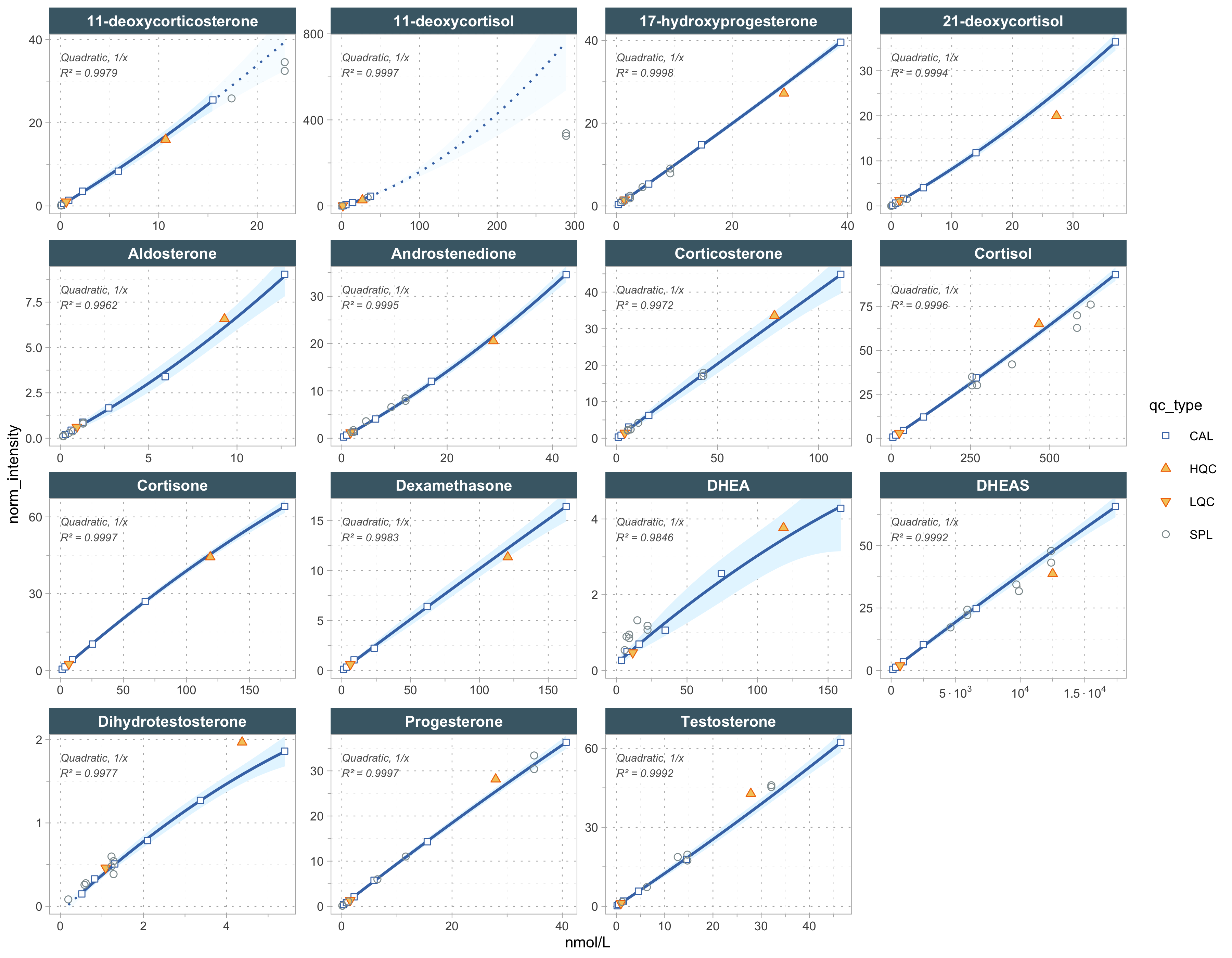
Each feature is normalized to its stable-isotope-labelled internal standard, then a quadratic, 1/x-weighted external calibration curve is fitted per analyte from the Cal 0–Cal F levels.
mexp <- normalize_by_istd(mexp)
#> ✔ 15 features normalized with 15 ISTDs in 30 analyses.
mexp <- calc_calibration_results(
mexp, fit_overwrite = TRUE, fit_model = "quadratic", fit_weighting = "1/x")
#> ✔ Calibration curve fits calculated for all 15 quantifier features. Average r-squared: 0.9978.The fitted curves and their metrics are inspected before quantification.
plot_calibrationcurves(
mexp, fit_overwrite = FALSE, fit_model = "quadratic", fit_weighting = "1/x",
include_istd = FALSE, include_qualifier = FALSE, show_progress = FALSE)
#> ✔ Calibration curve fits calculated for all 15 quantifier features. Average r-squared: 0.9978.
#> Generating plots (1 page)...#> done!
get_calibration_metrics(mexp) |>
filter(is_quantifier) |>
transmute(analyte = feature_id, fit_model, fit_weighting,
r2 = round(r2, 5), lod = signif(lod, 3), loq = signif(loq, 3))
#> # A tibble: 15 × 6
#> analyte fit_model fit_weighting r2 lod loq
#> <chr> <chr> <chr> <dbl> <dbl> <dbl>
#> 1 11-deoxycorticosterone quadratic 1/x 0.998 0.44 1.33
#> 2 11-deoxycortisol quadratic 1/x 1.000 0.273 0.826
#> 3 17-hydroxyprogesterone quadratic 1/x 1.000 0.196 0.593
#> 4 21-deoxycortisol quadratic 1/x 0.999 0.414 1.25
#> 5 Aldosterone quadratic 1/x 0.996 0.577 1.75
#> 6 Androstenedione quadratic 1/x 0.999 0.431 1.31
#> 7 Corticosterone quadratic 1/x 0.997 1.25 3.79
#> 8 Cortisol quadratic 1/x 1.000 1.22 3.71
#> 9 Cortisone quadratic 1/x 1.000 0.464 1.41
#> 10 DHEA quadratic 1/x 0.985 3.04 9.23
#> 11 DHEAS quadratic 1/x 0.999 8.29 25.1
#> 12 Dexamethasone quadratic 1/x 0.998 1.19 3.6
#> 13 Dihydrotestosterone quadratic 1/x 0.998 0.215 0.651
#> 14 Progesterone quadratic 1/x 1.000 0.252 0.765
#> 15 Testosterone quadratic 1/x 0.999 0.454 1.38Quantification
Concentrations are computed from the normalized intensities via the calibration curves. Qualifier transitions are excluded; analytes whose curve failed to fit are skipped rather than aborting the run.
mexp <- quantify_by_calibration(
mexp, fit_overwrite = FALSE, include_qualifier = FALSE,
ignore_failed_calibration = TRUE, fit_model = "quadratic", fit_weighting = "1/x")
#> ✔ Calibration curve fits calculated for all 15 quantifier features. Average r-squared: 0.9978.
#> ✔ Concentrations of these features were calculated for 30 analyses.
#> ℹ Concentrations are given in nmol/L.
# Export + reload the concentration table (wide: analysis_id, qc_type, analytes).
conc_path <- file.path("output", "Dataset4_quant_results.csv")
save_dataset_csv(mexp, path = conc_path, variable = "conc", add_qctype = TRUE)
#> ✔ Concentration values for 30 analyses and 15 features have been exported to 'output/Dataset4_quant_results.csv'.
d_conc_raw <- read_csv(conc_path, show_col_types = FALSE)MassHunter re-integration
The MassHunter Quantitative Analysis export is imported as a second experiment and reshaped to one tidy table — the single MassHunter source for all comparisons below. The trailing (ISTD) suffix on labelled internal standards is stripped so feature identifiers match MRMhub.
mh_reint <- import_data_masshunter(
MRMhubExperiment(title = "MassHunter re-integration"),
path = file.path(d4, "Dataset4_MassHunter-V2.csv"),
import_metadata = TRUE, silent = TRUE)
#> ℹ `feature_area` selected as default feature intensity. Modify with `set_intensity_var()`.
#> ✔ Analysis metadata associated with 30 analyses.
#> ✔ Feature metadata associated with 30 features.
mh_data <- get_analyticaldata(mh_reint, annotated = FALSE) |>
transmute(analysis_id,
feature_id = str_remove(feature_id, "[ ]*\\(ISTD\\)$"),
rt_mh = feature_rt,
area_mh = feature_area,
conc_mh = feature_conc_final)Below-Cal-A exclusion for study samples
Study samples (SPL = the SKML EQA samples) whose quantifier peak area falls below the corresponding Cal A area are below the lowest non-zero calibrator and treated as not reliably quantifiable. The rule is applied per analyte and independently per method — MRMhub SPL area vs MRMhub Cal A area, MassHunter SPL area vs MassHunter Cal A area — yielding the flags excl_mrm / excl_mh that downstream comparisons apply to their SPL rows. Internal standards are never filtered.
CAL_A_ID <- "Cal A_P1"
# MRMhub quantifier areas (quantifiers only, excluding the ISTDs).
mrm_q_area <- get_analyticaldata(mexp, annotated = TRUE) |>
filter(is_quantifier, !is_istd) |>
transmute(analysis_id, analyte_id = feature_id, qc_type, area_mrm = feature_area)
cala_mrm <- mrm_q_area |>
filter(analysis_id == CAL_A_ID) |>
select(analyte_id, cala_area_mrm = area_mrm)
cala_mh <- mh_data |>
filter(analysis_id == CAL_A_ID) |>
transmute(analyte_id = feature_id, cala_area_mh = area_mh)
# One row per SPL (analysis, analyte); flag below-Cal-A per method (NA-safe).
spl_area_excl <- mrm_q_area |>
filter(qc_type == "SPL") |>
left_join(select(mh_data, analysis_id, analyte_id = feature_id, area_mh),
by = c("analysis_id", "analyte_id")) |>
left_join(cala_mrm, by = "analyte_id") |>
left_join(cala_mh, by = "analyte_id") |>
mutate(excl_mrm = !is.na(area_mrm) & !is.na(cala_area_mrm) & area_mrm < cala_area_mrm,
excl_mh = !is.na(area_mh) & !is.na(cala_area_mh) & area_mh < cala_area_mh) |>
select(analysis_id, analyte_id, area_mrm, area_mh,
cala_area_mrm, cala_area_mh, excl_mrm, excl_mh)Low / high QC
Quantified concentrations of the low and high QC samples, one row per analyte.
d_conc_raw |>
filter(qc_type == "QC") |>
pivot_longer(!c(analysis_id, qc_type), names_to = "analyte", values_to = "conc") |>
mutate(qc = if_else(str_detect(analysis_id, "High"), "QC_High", "QC_Low")) |>
select(analyte, qc, conc) |>
pivot_wider(names_from = qc, values_from = conc) |>
mutate(across(where(is.numeric), ~ signif(.x, 3)))
#> # A tibble: 0 × 1
#> # ℹ 1 variable: analyte <chr>MRMhub vs MassHunter — Peak Integration
Figure 1 compares MRMhub-INTEGRATOR peak areas with the MassHunter re-integration of the same raw files. MRMhub quantifier and ISTD peaks are joined to MassHunter on analysis_id + feature_id, dropping near-noise peaks (area < 100), empty CAL rows, and below-Cal-A SPL points.
# Manuscript house theme + palettes (shared by both figures).
theme_set(theme_bw(base_size = 8, base_family = "sans") +
theme(panel.grid.minor = element_blank(),
legend.position = "bottom",
plot.title = element_text(size = 8, face = "plain"),
legend.key.size = unit(3.2, "mm"),
legend.margin = margin(1, 1, 1, 1)))
col_method <- c(MRMhub = "#2C7FB8", MassHunter = "#D95F0E")
smp_cols <- c(CAL = "#0072B2", HQC = "#D55E00", LQC = "#E69F00",
SPL = "grey30", SST = "#009E73", SBLK = "#CC79A7", PBLK = "#999999")
# Save a composite as vector PDF + 300-dpi PNG at a given size (mm) for the manuscript.
save_fig <- function(plot, stem, height, width = 180) {
ggsave(file.path("output", paste0(stem, ".pdf")), plot,
device = cairo_pdf, width = width, height = height, units = "mm")
ggsave(file.path("output", paste0(stem, ".png")), plot,
device = ragg::agg_png, width = width, height = height, units = "mm", dpi = 300)
invisible(plot)
}mrm_peaks_q <- get_analyticaldata(mexp, annotated = TRUE) |>
filter(is_quantifier | is_istd) |>
transmute(analysis_id, feature_id, qc_type, sample_id,
feature_type = factor(if_else(is_istd, "ISTD", "Quantifier"),
levels = c("Quantifier", "ISTD")),
rt_mrm = feature_rt, area_mrm = feature_area)
d_peakcmp_reint <- mrm_peaks_q |>
inner_join(mh_data, by = c("analysis_id", "feature_id")) |>
filter(!is.na(rt_mrm), !is.na(rt_mh), !is.na(area_mrm), !is.na(area_mh)) |>
filter(area_mrm >= 100, area_mh >= 100) |>
filter(!(qc_type == "CAL" & is.na(sample_id) & feature_type != "ISTD")) |>
left_join(select(spl_area_excl, analysis_id, analyte_id, excl_mrm, excl_mh),
by = c("analysis_id", "feature_id" = "analyte_id")) |>
filter(!(qc_type == "SPL" &
(coalesce(excl_mrm, FALSE) | coalesce(excl_mh, FALSE)))) |>
select(-excl_mrm, -excl_mh) |>
mutate(area_diff_pct = (area_mh - area_mrm) / area_mrm * 100,
rt_diff = rt_mh - rt_mrm,
subset = case_when(
analysis_id %in% sst_analysis_ids ~ "SST",
analysis_id %in% assay_analysis_ids ~ "ASSAY",
TRUE ~ NA_character_))Peak-area agreement
Log–log peak areas against the 1:1 line (Pearson r on log10 values). CAL/QC/SST samples span four orders of magnitude; agreement is essentially exact.
smp_lv <- c("CAL", "HQC", "LQC", "SST")
smp_cols4 <- c(CAL = "#0072B2", HQC = "#D55E00", LQC = "#E69F00", SST = "#009E73")
ft_shapes <- c(Quantifier = 16, ISTD = 17)
scale_smp <- scale_colour_manual(values = smp_cols4, limits = smp_lv, drop = FALSE)
scale_ft <- scale_shape_manual(values = ft_shapes)
d_cmp <- d_peakcmp_reint |>
filter(qc_type %in% smp_lv) |>
mutate(qc_type = factor(qc_type, levels = smp_lv))
r_log <- cor(log10(d_cmp$area_mrm), log10(d_cmp$area_mh))
ax_lims <- range(c(d_cmp$area_mrm, d_cmp$area_mh))
p_corr <- d_cmp |>
ggplot(aes(area_mrm, area_mh, colour = qc_type, shape = feature_type)) +
geom_abline(slope = 1, intercept = 0, linetype = "dashed", colour = "grey40") +
geom_point(size = 1.1, alpha = 0.7) +
annotate("text", x = ax_lims[1], y = ax_lims[2], hjust = 0, vjust = 1, size = 2.4,
label = sprintf("Pearson r = %.4f", r_log)) +
scale_x_log10(limits = ax_lims) + scale_y_log10(limits = ax_lims) +
scale_smp + scale_ft +
guides(colour = guide_legend(order = 1, nrow = 2),
shape = guide_legend(order = 2, nrow = 2)) +
labs(x = "MRMhub peak area", y = "MassHunter peak area",
colour = "Sample type", shape = "Feature", title = "Peak-area agreement")
p_corrPrecision (%CV) equivalence
Per-feature %CV over the ten replicate SST injections, MRMhub vs MassHunter. The two methods deliver equivalent precision (points on the 1:1 line).
sst_cv <- d_peakcmp_reint |>
filter(subset == "SST") |>
group_by(feature_type, feature_id) |>
summarise(cv_mrmhub = sd(area_mrm) / mean(area_mrm) * 100,
cv_masshunter = sd(area_mh) / mean(area_mh) * 100,
.groups = "drop")
cv_lims <- range(c(sst_cv$cv_mrmhub, sst_cv$cv_masshunter)) + c(-0.3, 0.3)
p_cv <- sst_cv |>
ggplot(aes(cv_mrmhub, cv_masshunter, shape = feature_type)) +
geom_abline(slope = 1, intercept = 0, linetype = "dashed", colour = "grey60") +
geom_point(size = 1.6, alpha = 0.85, colour = "#009E73") +
coord_cartesian(xlim = cv_lims, ylim = cv_lims) + scale_ft +
guides(shape = "none") +
labs(x = "MRMhub %CV (10 SST reps)", y = "MassHunter %CV",
title = "Precision (%CV) equivalence")
p_cvBland–Altman
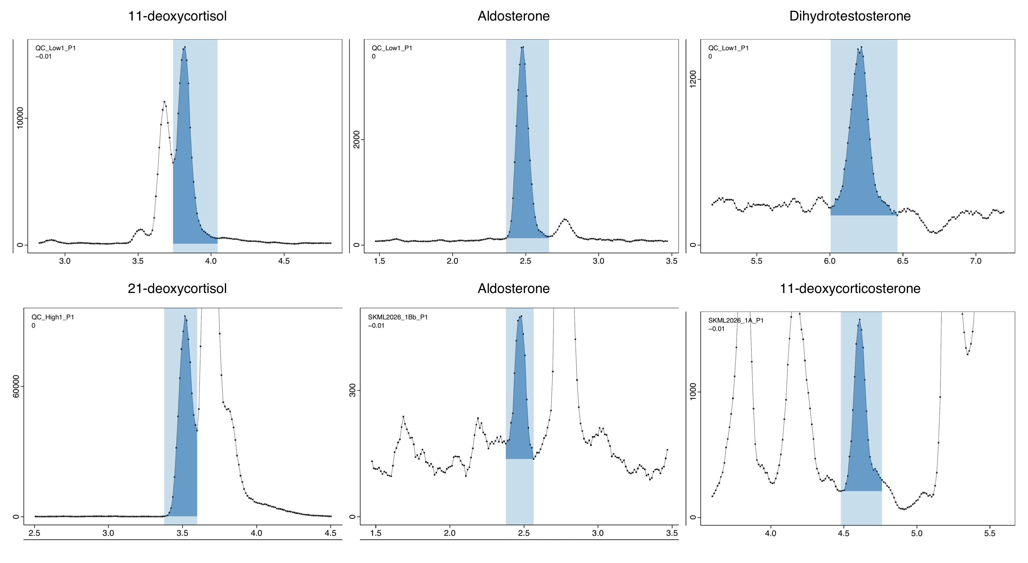
Percent difference (MassHunter − MRMhub) against the mean area, excluding SST and near-noise peaks (mean area < 10³). The three analytes highlighted here have the largest real-sample differences and their chromatograms are shown below.
highlight_analytes <- c("21-deoxycortisol", "11-deoxycortisol", "Aldosterone")
hl_cols <- setNames(c("#D81B60", "#1E88E5", "#8E44AD"), highlight_analytes)
d_ba <- d_peakcmp_reint |>
filter(qc_type != "SST") |>
mutate(mean_area = (area_mrm + area_mh) / 2,
pct_diff = (area_mh - area_mrm) / mean_area * 100,
hl = factor(if_else(feature_id %in% highlight_analytes, feature_id, NA_character_),
levels = highlight_analytes)) |>
filter(mean_area >= 1e3)
ba_bias <- mean(d_ba$pct_diff)
ba_loa <- ba_bias + c(-1.96, 1.96) * sd(d_ba$pct_diff)
ba_xr <- max(d_ba$mean_area)
p_ba <- d_ba |>
ggplot(aes(mean_area, pct_diff)) +
geom_hline(yintercept = 0, colour = "grey70") +
geom_hline(yintercept = ba_bias, colour = "grey20") +
geom_hline(yintercept = ba_loa, linetype = "dashed", colour = "grey50") +
geom_point(data = ~ filter(.x, is.na(hl)), colour = "grey80", size = 0.9, alpha = 0.6) +
geom_point(data = ~ filter(.x, !is.na(hl)), aes(colour = hl), size = 1.7, alpha = 0.9) +
annotate("text", x = ba_xr, y = ba_bias, hjust = 1, vjust = -0.6, size = 2.1,
colour = "grey20", label = sprintf("mean bias %.1f%%", ba_bias)) +
annotate("text", x = ba_xr, y = ba_loa[2], hjust = 1, vjust = 1.4, size = 2,
colour = "grey45", label = "+95% LoA") +
annotate("text", x = ba_xr, y = ba_loa[1], hjust = 1, vjust = -0.7, size = 2,
colour = "grey45", label = "-95% LoA") +
scale_colour_manual(values = hl_cols, name = "Highlighted analyte", na.translate = FALSE) +
scale_x_log10(limits = c(1e3, NA)) + coord_cartesian(ylim = c(-20, 20)) +
labs(x = "Mean peak area of the two methods (>= 10^3)",
y = "Percent difference (MH - MRMhub) %",
title = sprintf("Bland-Altman (excl. SST, area >= 10^3): mean bias %.1f%%, 95%% LoA [%.0f, %.0f]%%",
ba_bias, ba_loa[1], ba_loa[2]))
p_baExample chromatograms
The largest real-sample area differences occur where a peak sits on an elevated baseline or beside a co-eluting neighbour, so the integration boundaries — and hence the areas — legitimately differ between the two integrators. The candidate table ranks these cases; the panel crops the three chosen examples (one per highlighted analyte) from the MRMhub by_transition chromatograms.
chrom_candidates <- d_peakcmp_reint |>
filter(feature_type == "Quantifier",
qc_type %in% c("CAL", "HQC", "LQC", "SPL", "SST"),
area_mrm >= 20000) |>
arrange(desc(abs(area_diff_pct))) |>
transmute(feature_id, analysis_id, qc_type,
area_mrm = round(area_mrm), area_mh = round(area_mh),
area_diff_pct = round(area_diff_pct, 1)) |>
head(10)
chrom_candidates
#> # A tibble: 10 × 6
#> feature_id analysis_id qc_type area_mrm area_mh area_diff_pct
#> <chr> <chr> <chr> <dbl> <dbl> <dbl>
#> 1 21-deoxycortisol SKML2025_6B_P1 SPL 34372 42059 22.4
#> 2 17-hydroxyprogesterone SKML2025_6B_P1 SPL 76446 59981 -21.5
#> 3 11-deoxycortisol SKML2026_2B_P1 SPL 45558 40661 -10.7
#> 4 Dihydrotestosterone Cal D_P1 CAL 22013 24289 10.3
#> 5 DHEA 20260212_SST03 SST 42897 38529 -10.2
#> 6 DHEA Cal D_P1 CAL 81165 88766 9.4
#> 7 11-deoxycortisol 20260212_SST07 SST 1285343 1389585 8.1
#> 8 Androstenedione Cal A_P1 CAL 76008 81960 7.8
#> 9 DHEA Cal E_P1 CAL 197230 212468 7.7
#> 10 17-hydroxyprogesterone SKML2026_2Ab_P1 SPL 127355 137090 7.6# Panel-D chromatograms are the pre-generated crops (see the INTEGRATOR section);
# subtitles carry the data-derived area difference for each example.
chrom_examples <- tibble::tribble(
~name, ~feature_id, ~analysis_id,
"fig1d_21-deoxycortisol", "21-deoxycortisol", "SKML2025_6B_P1",
"fig1d_11-deoxycortisol", "11-deoxycortisol", "SKML2026_2B_P1",
"fig1d_Aldosterone", "Aldosterone", "SKML2026_2A_P1")
chrom_meta <- chrom_examples |>
left_join(distinct(d_peakcmp_reint, feature_id, analysis_id, area_diff_pct),
by = c("feature_id", "analysis_id")) |>
mutate(subtitle = sprintf("%s (dArea %+.1f%%)",
str_remove(analysis_id, "_P1$"), area_diff_pct))
chrom_plots <- Map(chrom_gg, chrom_meta$name, chrom_meta$feature_id, chrom_meta$subtitle)
p_chrom <- wrap_elements(full = wrap_plots(chrom_plots, nrow = 1))
p_chromFigure 1 — manuscript figure
The four panels above are composed into the publication figure (Figure 1) and saved as a vector PDF and a 300-dpi PNG (Nature 180 mm width).
row_ab <- (p_corr + p_cv) + plot_layout(guides = "collect") &
theme(legend.position = "bottom")
fig1 <- row_ab / p_ba / p_chrom +
plot_layout(heights = c(1, 0.72, 0.58)) +
plot_annotation(tag_levels = "A")
save_fig(fig1, "fig1_integration_correspondence", height = 230)
fig1output/fig1_integration_correspondence.{pdf,png} (180 mm).MRMhub vs MassHunter — Quantification
Figure 2 compares the two pipelines at the quantification stage. To isolate the post-processing (calibration + quantification) from the peak integration, we also feed MassHunter’s own peak areas through the MRMhub pipeline — identical areas, identical calibration model — so any concentration difference is due to post-processing alone.
mh_area <- mh_data |> transmute(analysis_id, feature_name = feature_id, area_mh)
long_mh <- read_csv(long_combined_path, show_col_types = FALSE) |>
mutate(.aid = str_remove(raw_data_filename, "[.]mzML$")) |>
inner_join(mh_area, by = c(".aid" = "analysis_id", "feature_name")) |>
mutate(area = area_mh) |>
select(-.aid, -area_mh)
tmp_long <- tempfile(fileext = ".csv")
write_csv(long_mh, tmp_long)
mexp_mh <- MRMhubExperiment(title = "MassHunter areas via MRMhub pipeline")
mexp_mh <- import_data_mrmhub(mexp_mh, path = tmp_long, import_metadata = TRUE)
#> ✔ Imported 30 analyses with 30 features
#> ℹ `feature_area` selected as default feature intensity. Modify with `set_intensity_var()`.
#> ✔ Analysis metadata associated with 30 analyses.
#> ✔ Feature metadata associated with 30 features.
mexp_mh <- import_metadata_msorganiser(
mexp_mh, path = meta_path, excl_unmatched_analyses = TRUE, ignore_warnings = TRUE)
#> ! Metadata has following warnings and notifications:
#> --------------------------------------------------------------------------------------------
#> Type Table Column Issue Count
#> 1 N Analyses sample_id Not defined for all analyses 16
#> 2 W* Analyses analysis_id Analyses not in analysis data 3
#> 3 N Features analyte_id Not defined for all features 15
#> --------------------------------------------------------------------------------------------
#> E = Error, W = Warning, W* = Supressed Warning, N = Note
#> --------------------------------------------------------------------------------------------
#> ✔ Analysis metadata associated with 30 analyses.
#> ✔ Feature metadata associated with 30 features.
#> ✔ Internal Standard metadata associated with 15 ISTDs.
#> ✔ QC concentration metadata associated with 13 annotated samples and 15 annotated analytes
mexp_mh <- normalize_by_istd(mexp_mh)
#> ✔ 15 features normalized with 15 ISTDs in 30 analyses.
mexp_mh <- calc_calibration_results(mexp_mh, fit_overwrite = TRUE,
fit_model = "quadratic", fit_weighting = "1/x")
#> ✔ Calibration curve fits calculated for all 15 quantifier features. Average r-squared: 0.9963.
mexp_mh <- quantify_by_calibration(mexp_mh, fit_overwrite = FALSE,
include_qualifier = FALSE,
ignore_failed_calibration = TRUE,
fit_model = "quadratic", fit_weighting = "1/x")
#> ✔ Calibration curve fits calculated for all 15 quantifier features. Average r-squared: 0.9963.
#> ✔ Concentrations of these features were calculated for 30 analyses.
#> ℹ Concentrations are given in nmol/L.Calibration fit comparison
Calibration R² per analyte: MassHunter’s own fit vs the MRMhub full-pipeline fit.
mh_own_r2 <- read_csv(file.path(d4, "Dataset4_MassHunter-CalibrationFits.csv"),
show_col_types = FALSE) |>
transmute(analyte_id, r2_mh_own = r2)
r2_cmp <- get_calibration_metrics(mexp_mh) |>
filter(is_quantifier) |>
transmute(analyte_id = feature_id, r2_mrmpipe_mharea = r2) |>
left_join(mh_own_r2, by = "analyte_id") |>
left_join(get_calibration_metrics(mexp) |> filter(is_quantifier) |>
transmute(analyte_id = feature_id, r2_mrmpipe_mrmarea = r2),
by = "analyte_id")
chain_lv <- c("MassHunter", "MRMhub")
chain_col <- c(MassHunter = "#D95F0E", MRMhub = "#2C7FB8")
ord_r2 <- r2_cmp |> arrange(r2_mrmpipe_mrmarea) |> pull(analyte_id)
d_r2_long <- r2_cmp |>
transmute(analyte_id, MassHunter = r2_mh_own, MRMhub = r2_mrmpipe_mrmarea) |>
pivot_longer(-analyte_id, names_to = "chain", values_to = "r2") |>
mutate(analyte_id = factor(analyte_id, levels = ord_r2),
chain = factor(chain, levels = chain_lv))
# Truncate the x-axis just below the dense 0.996–1.000 cluster; flag off-scale rows.
R2_FLOOR <- 0.9955
r2_off <- d_r2_long |> filter(r2 < R2_FLOOR) |> distinct(analyte_id) |>
mutate(r2 = R2_FLOOR)
off_txt <- d_r2_long |> filter(r2 < R2_FLOOR) |>
group_by(analyte_id) |> summarise(v = min(r2), .groups = "drop") |>
arrange(v) |> mutate(t = sprintf("%s %.3f", analyte_id, v))
p_r2 <- ggplot(d_r2_long, aes(r2, analyte_id)) +
geom_line(aes(group = analyte_id), colour = "grey75", linewidth = 0.6) +
geom_point(aes(colour = chain), size = 1.9, alpha = 0.9) +
geom_text(data = r2_off, aes(label = "<"), hjust = 0, nudge_x = 0.00004,
size = 2.3, colour = "grey45") +
scale_colour_manual(values = chain_col, name = NULL) +
scale_x_continuous(breaks = c(0.996, 0.997, 0.998, 0.999, 1.000)) +
coord_cartesian(xlim = c(R2_FLOOR, 1.0004)) +
labs(x = expression(Calibration~R^2), y = NULL, title = "Calibration curve fit comparison",
subtitle = paste0("x-axis truncated at ", R2_FLOOR,
"; off scale (<): ", paste(off_txt$t, collapse = ", "))) +
theme(plot.subtitle = element_text(size = 6.5, colour = "grey30"),
plot.margin = margin(4, 10, 4, 4),
legend.position = "inside", legend.position.inside = c(0.015, 0.98),
legend.justification.inside = c(0, 1),
legend.background = element_rect(fill = alpha("white", 0.7), colour = NA),
legend.key.size = unit(3, "mm"))
p_r2Concentration equivalence on identical areas
Feeding MassHunter areas through the MRMhub pipeline reproduces MassHunter’s end-to-end concentrations almost exactly — the post-processing steps are equivalent.
tmp_conc <- tempfile(fileext = ".csv")
save_dataset_csv(mexp_mh, path = tmp_conc, variable = "conc", add_qctype = TRUE)
#> ✔ Concentration values for 30 analyses and 15 features have been exported to '/var/folders/3r/ywcsb3896zj4_0xlb_70yvlh0000gn/T//RtmprtMdZS/file6bc310f68e2f.csv'.
d_qonly <- read_csv(tmp_conc, show_col_types = FALSE) |>
pivot_longer(!c(analysis_id, qc_type), names_to = "analyte_id",
values_to = "conc_mrmpipe") |>
left_join(mh_data |> select(analysis_id, analyte_id = feature_id, conc_mh),
by = c("analysis_id", "analyte_id")) |>
filter(!is.na(conc_mrmpipe), !is.na(conc_mh)) |>
filter(!qc_type %in% c("SBLK", "PBLK")) |>
mutate(qc_type = factor(qc_type, levels = names(smp_cols)))
posq <- d_qonly |> filter(conc_mrmpipe > 0, conc_mh > 0)
q_r <- cor(log10(posq$conc_mrmpipe), log10(posq$conc_mh))
q_med <- median(abs((d_qonly$conc_mrmpipe - d_qonly$conc_mh) / d_qonly$conc_mh * 100))
axq <- range(c(posq$conc_mrmpipe, posq$conc_mh))
p_qonly <- posq |>
ggplot(aes(conc_mh, conc_mrmpipe, colour = qc_type)) +
geom_abline(slope = 1, intercept = 0, linetype = "dashed", colour = "grey40") +
geom_point(size = 1.1, alpha = 0.6) +
annotate("text", x = axq[1], y = axq[2], hjust = 0, vjust = 1, size = 2.4,
label = sprintf("Pearson r = %.5f\nmedian |d| = %.3f%%", q_r, q_med)) +
scale_x_log10(limits = axq) + scale_y_log10(limits = axq) +
scale_colour_manual(values = smp_cols, drop = TRUE, name = "Sample type") +
coord_equal() +
labs(x = "MassHunter End-to-End", y = "MRMhub-QUANT on MH areas",
title = "Concentration equivalence (same areas)") +
theme(legend.position = "inside", legend.position.inside = c(0.98, 0.02),
legend.justification.inside = c(1, 0),
legend.background = element_rect(fill = alpha("white", 0.7), colour = NA),
legend.key.size = unit(2.8, "mm"),
legend.title = element_text(size = 6.5), legend.text = element_text(size = 6))
p_qonlyFull end-to-end concentration agreement
Independent end-to-end concentrations (each method’s own integration and calibration) for the LQC, HQC and SPL samples.
d_full <- d_conc_raw |>
filter(qc_type %in% c("LQC", "HQC", "SPL")) |>
pivot_longer(!c("analysis_id", "qc_type"), names_to = "analyte_id", values_to = "conc") |>
left_join(mh_data |> select(analysis_id, analyte_id = feature_id, conc_mh),
by = c("analysis_id", "analyte_id")) |>
left_join(select(spl_area_excl, analysis_id, analyte_id, excl_mrm, excl_mh),
by = c("analysis_id", "analyte_id")) |>
mutate(conc = if_else(coalesce(excl_mrm, FALSE), NA_real_, conc),
conc_mh = if_else(coalesce(excl_mh, FALSE), NA_real_, conc_mh)) |>
select(-excl_mrm, -excl_mh) |>
filter(!is.na(conc), !is.na(conc_mh), conc > 0, conc_mh > 0) |>
mutate(qc_type = factor(qc_type, levels = names(smp_cols)))
f_r <- cor(log10(d_full$conc), log10(d_full$conc_mh))
f_med <- median(abs((d_full$conc - d_full$conc_mh) / d_full$conc_mh * 100))
axf <- range(c(d_full$conc, d_full$conc_mh))
p_full <- d_full |>
ggplot(aes(conc_mh, conc, colour = qc_type)) +
geom_abline(slope = 1, intercept = 0, linetype = "dashed", colour = "grey40") +
geom_point(size = 1.3, alpha = 0.7) +
annotate("text", x = axf[1], y = axf[2], hjust = 0, vjust = 1, size = 2.4,
label = sprintf("Pearson r = %.4f\nmedian |d| = %.1f%%", f_r, f_med)) +
scale_x_log10(limits = axf) + scale_y_log10(limits = axf) +
scale_colour_manual(values = smp_cols, drop = TRUE, name = "Sample type") +
coord_equal() +
labs(x = "MassHunter (end-to-end)", y = "MRMhub (end-to-end)",
title = "Concentration agreement (full pipeline)") +
theme(legend.position = "none")
p_fullEQA accuracy against SKML reference values
Per-analyte percent bias against the SKML EQA reference concentrations, one point per EQA sample per method (dashed lines: ±15 %). The reference concentrations are read from the metadata workbook’s QC Concentrations sheet (imported above with the rest of the metadata), keyed by sample and analyte. DHEA and DHEAS are excluded (large biases that would compress the other panels).
# EQA target concentrations come from the metadata's `QC Concentrations` sheet
# (imported above), keyed by `sample_id` + `analyte_id`. They surface via the
# `annot_qcconcentrations` slot; DHEAS is already stored in nmol/L there.
eqa_target <- mexp@annot_qcconcentrations |>
filter(str_starts(sample_id, "SKML")) |>
transmute(sample_id, analyte_id, target = concentration)
# analysis_id -> sample_id map (groups the `…b` replicates onto one EQA sample).
sid_map <- get_analyticaldata(mexp, annotated = TRUE) |>
distinct(analysis_id, sample_id)
d_eqa <- d_conc_raw |>
filter(qc_type == "SPL") |>
pivot_longer(!c("analysis_id", "qc_type"), names_to = "analyte_id", values_to = "conc_mrm") |>
left_join(mh_data |> select(analysis_id, analyte_id = feature_id, conc_mh),
by = c("analysis_id", "analyte_id")) |>
left_join(select(spl_area_excl, analysis_id, analyte_id, excl_mrm, excl_mh),
by = c("analysis_id", "analyte_id")) |>
mutate(conc_mrm = if_else(coalesce(excl_mrm, FALSE), NA_real_, conc_mrm),
conc_mh = if_else(coalesce(excl_mh, FALSE), NA_real_, conc_mh)) |>
left_join(sid_map, by = "analysis_id") |>
inner_join(eqa_target, by = c("sample_id", "analyte_id")) |>
# Compact axis label, e.g. SKML2026_1A -> 2026.1A.
mutate(sample_eqa = str_replace(str_remove(sample_id, "^SKML"), "^([0-9]{4})_", "\\1.")) |>
transmute(analyte_id, sample_eqa, analysis_id, target, conc_mrm, conc_mh,
bias_mrmhub = (conc_mrm - target) / target * 100,
bias_masshunter = (conc_mh - target) / target * 100) |>
filter(!(is.na(conc_mrm) & is.na(conc_mh)))
p_eqa <- d_eqa |>
filter(!analyte_id %in% c("DHEA", "DHEAS")) |>
pivot_longer(c(bias_mrmhub, bias_masshunter), names_to = "method", values_to = "bias") |>
filter(!is.na(bias)) |>
mutate(method = recode(method, bias_mrmhub = "MRMhub", bias_masshunter = "MassHunter"),
method = factor(method, levels = c("MRMhub", "MassHunter"))) |>
ggplot(aes(sample_eqa, bias, colour = method, shape = method)) +
geom_hline(yintercept = 0, colour = "grey40") +
geom_hline(yintercept = c(-15, 15), linetype = "dashed", colour = "grey75") +
geom_point(size = 1.5, alpha = 0.85, position = position_dodge(width = 0.4)) +
scale_colour_manual(values = col_method, name = "Method") +
scale_shape_manual(values = c(MRMhub = 16, MassHunter = 17), name = "Method") +
facet_wrap(vars(analyte_id), scales = "free_y", ncol = 4) +
labs(x = NULL, y = "Bias vs EQA reference (%)",
title = "EQA accuracy - bias per analyte (excl. DHEA, DHEAS)") +
theme(panel.grid.minor = element_blank(),
strip.text = element_text(size = 6),
axis.text.x = element_text(angle = 45, hjust = 1, size = 5),
axis.text.y = element_text(size = 5.2))
p_eqaFigure 2 — manuscript figure
The four panels above are composed into the publication figure (Figure 2).
fig2 <- p_r2 / (p_qonly + p_full) / p_eqa +
plot_layout(heights = c(0.68, 0.95, 1.2)) +
plot_annotation(tag_levels = "A")
save_fig(fig2, "fig2_quantification_comparison", height = 220)
fig2output/fig2_quantification_comparison.{pdf,png} (180 mm).