if (!require("pak")) install.packages("pak")
# This site was rendered with mrmhub 0.9.9 (the QUANT module of MRMhub),
# installed from its default branch (main).
pak::pak("SLINGhub/MRMhub")

# Parallel processing (mirai), coloured console output (fansi), and the
# optional plotting packages used by some QC figures in this workflow.
pak::pak(c("mirai", "fansi", "ggvenn", "patchwork", "ggbeeswarm"))MRMhub Data Processing Workflow for Dataset 1
SPERFECT
1 Overview Dataset
The data come from the SPERFECT study (SPhingolipids as sErial biomaRkers oF disease progression in acutE myoCardial infarcTion; Tan et al. (2022)), a targeted lipidomics analysis of plasma from 84 participants at risk of coronary artery disease. Participants contributed to a longitudinal arm with blood collection at up to five follow-up time points (378 samples), and a subset to a diurnal rhythm study (299 samples). Including QC samples, the dataset comprises 937 injections acquired by LC-MRM in six analytical batches; 464 MRM transitions were monitored, from which 482 features were integrated (a transition can yield multiple features, e.g. for isomers or isobars). The QC samples are solvent blanks (SBLK), process blanks (PBLK, containing the ISTD mix), technical QC (TQC, pooled aliquots of extracted study samples), batch QC (BQC, aliquots of pooled plasma extracted alongside the study samples), response-curve QC (RQC, the TQC injected at different volumes) and long-term reference (LTR) samples. PBLKs and BQCs were co-extracted; PBLK, TQC and BQC samples were measured at regular intervals throughout the analysis to monitor background signal, instrument performance and overall process performance, respectively.
This example workflow covers the complete MRMhub data processing pipeline on this dataset: peak integration, quantitation, quality control and reporting. It includes many elements of the MRMhub workflow, some of which may not be applicable or necessary for other datasets.
Some plots are assigned to a variable (e.g. fig4a, fig4b) so they can be reused at the end of this workflow to assemble the multi-panel manuscript figures.
ImportantData availability
All code and data for this workflow are deposited in the Zenodo record 10.5281/zenodo.15370293 (MRMhub-workflows). The corresponding MS raw data (mzML files), together with the MRMhub-INTEGRATOR application and its input files, are deposited as MRMhub-Dataset1.zip in the same record.
2 Raw Data Processing: Peak Picking and Integration
Peak picking and peak integration were performed with MRMhub-INTEGRATOR. For more details on the usage of the INTEGRATOR application, see the INTEGRATOR Manual.
2.1 Conversion of vendor raw files to mzML
INTEGRATOR requires the raw files to be in the mzML format. The original raw data files (Agilent .d) were converted to mzML using msconvert from the ProteoWizard software (https://proteowizard.sourceforge.io) with the following settings: output format = mzML; binary encoding precision = 32 bit; write index = true. See the MRMhub Manual for more details.
2.2 Preparing the INTEGRATOR input files
INTEGRATOR requires three different input files. Templates and examples are included in the downloaded MRMhub-INTEGRATOR release archive. The final input files used for this dataset are contained in MRMhub-Dataset1.zip (see above), for those who wish to re-run the integration. The following subsections describe each required input file and the key settings used for this example.
2.2.1 Global Settings File
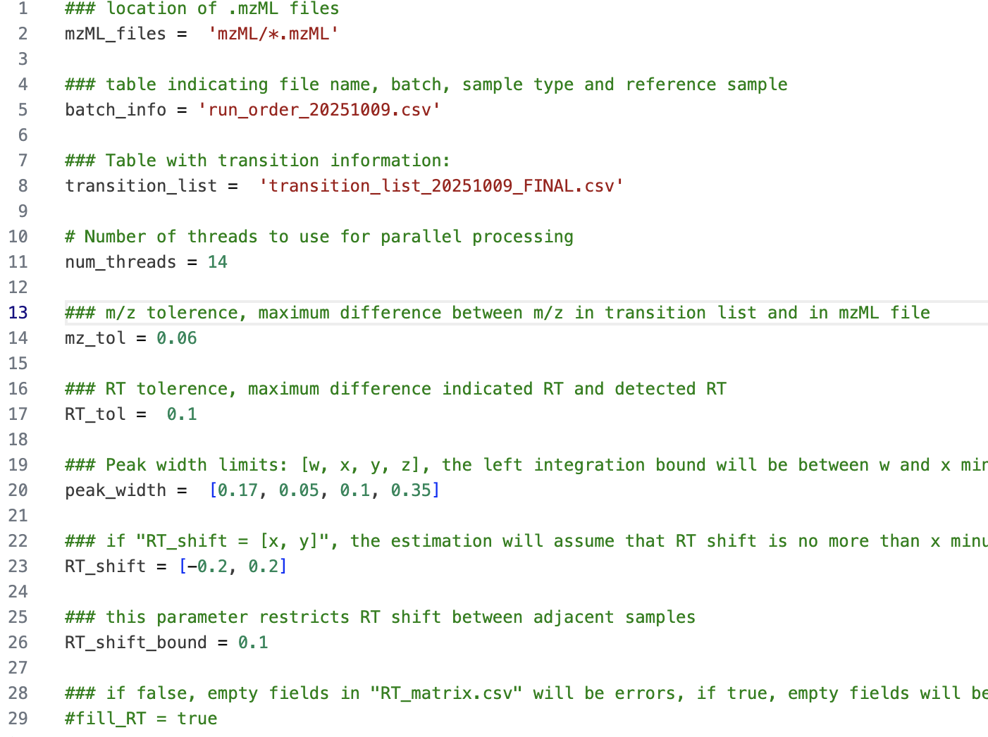
The parameter mz_tol, defining the maximum tolerance in m/z values for identifying transitions, was set to 0.06. The RT_tol parameter, defining the window around the expected RT (see Feature/Transition table below) in which features are searched, was set to 0.1 min. This relatively narrow RT window was chosen to reduce selection of incorrect peaks in complex chromatograms, as observed in this dataset. In this dataset peaks exhibited some tailing, thus the peak_width was set to [0.15, 0.5, 0.1, 0.35], with the right-side ranges set to longer than the left-side ranges. For specific features with broader or convoluted peaks, feature-specific peak widths were applied, overwriting the global settings (see Feature Table below). The maximum allowed RT shift correction was set to (-0.2, 0.2), and the maximum allowed sample-to-sample RT shift was 0.1 min. The full set of settings in param.txt is shown in the figure below.
2.2.2 Sample Table
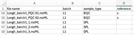
In the sample table (run_order_20251009.csv) the samples to be processed were listed by their .mzML file names. The first two BQC (batch quality control) samples were selected as retention time reference anchors. The sample type for each sample was defined in column C (sample_type) using the MRMhub QC type nomenclature. This is optional and INTEGRATOR distinguishes only between blanks (identified by the presence of the text BLK), and non-blanks.
2.2.3 Feature/Transition Table
The feature/transition table (transition_list_20251009.csv) defined the transitions to be extracted from the .mzML files by precursor and product m/z values. Each feature (peak or peak group) was specified by its expected retention time (RT, in minutes). For some transitions, multiple features were defined. The corresponding internal standard feature for each entry was included in the table, however, these internal standards were not used by INTEGRATOR but were exported in the integration results.

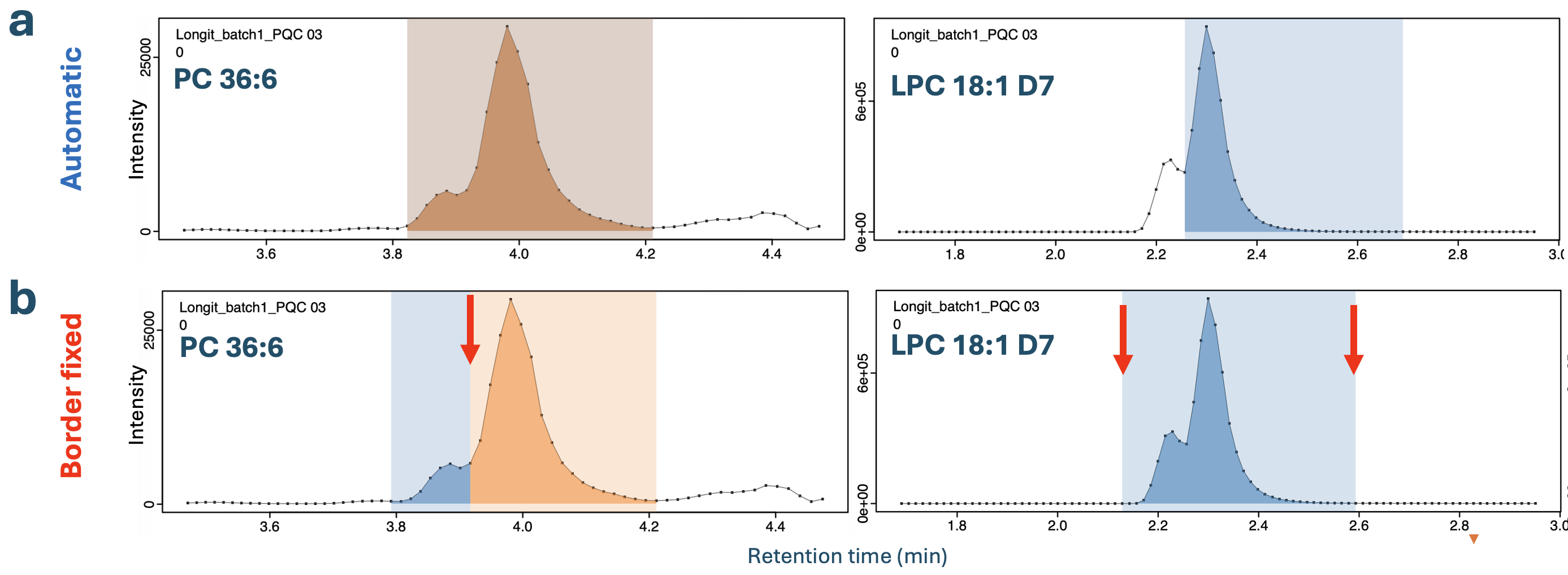
For this dataset, fixed borders were defined for some features that were poorly separated from adjacent peaks or that had noisy chromatograms to ensure correct and consistent integration, for example PC 36:6. In some other cases, isomers were intentionally co-integrated, such as the LPC and LPE internal standards (see Figure 4). The final version of the feature/transition table (transition_list_20251009_Final.csv) is the result from several rounds of parameter optimization with INTEGRATOR and from peak picking QC using the QUANT module, see below. INTEGRATOR continues to be developed, and some of these feature-specific settings may become unnecessary as the automated peak integration is improved.
2.3 Running MRMhub-INTEGRATOR and Review of Results
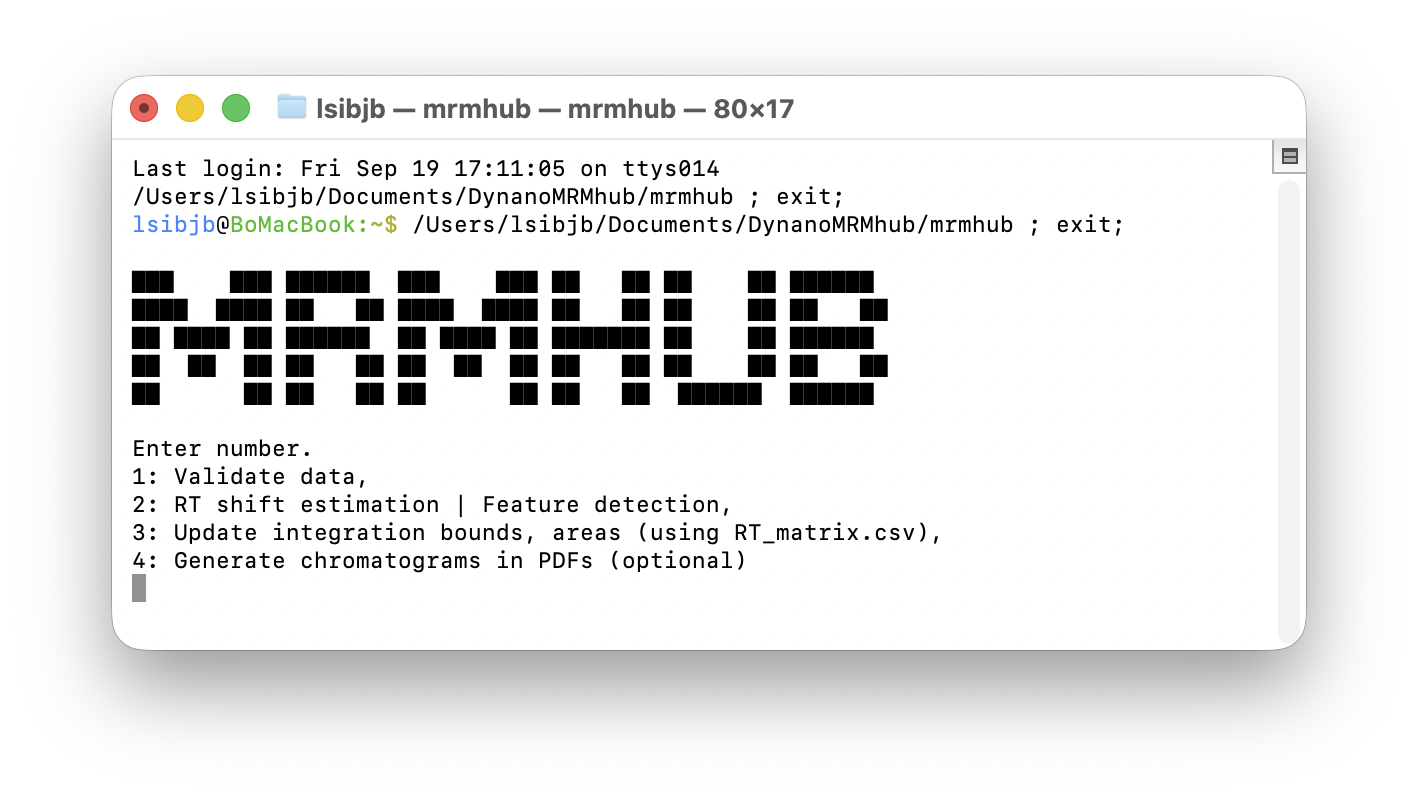
The most recent release of INTEGRATOR was obtained from https://github.com/SLINGhub/MRMhub/releases. After preparing all input files, the INTEGRATOR application is started. Steps 1 to 4 then run consecutively without further input to perform peak detection, peak picking, integration, and export of data and PDF results. The integration results are reported in the generated file ‘long.csv’, a long-format table that includes peak areas, actual retention time, peak width, and other metadata. This data file will be used for subsequent data postprocessing (see the following section). A wide-format table with peak areas is available as ‘quant_raw.csv’. PDFs of the integrated transitions are available in the by_* folders. See the INTEGRATOR Manual for more details.
The peak integration results were inspected for all features across samples using the generated PDFs (see above). In this dataset, RT shifts across the entire run of 937 samples were less than 0.02 min.
3 Data Postprocessing and QC
The postprocessing (Quantification, Quality Control and Reporting) of the data obtained from the peak integration above is conducted using MRMhub-QUANT, which is implemented as the {mrmhub} R package. A Quarto computational notebook is used to run, document and report the data postprocessing.
3.1 Setting up a Quarto Notebook and Installation of {mrmhub}
A Quarto notebook was created in RStudio. The {mrmhub} R package was installed by running the following code in the R console, together with the mirai (parallel processing) and fansi (coloured console output) packages, and the optional plotting packages (ggvenn, patchwork, ggbeeswarm) used in this workflow.
Notemrmhub version
These notebooks were rendered with mrmhub 0.9.9 (QUANT module of MRMhub, main branch); install with pak::pak("SLINGhub/MRMhub").
The Quarto notebook code generated in this example workflow is available from https://github.com/SLINGhub/MRMhub-workflows (file Dataset1.qmd). In the subsequent section, the data postprocessing is encoded and documented step-by-step into the notebook as individual code chunks using {mrmhub} functions.
3.2 Postprocessing workflow
3.2.1 Load mrmhub and other required packages
To improve performance, multi-threading was used for some of the calculations and plotting, for which the R package {mirai} needs to be installed and loaded.
library(mrmhub)

# Colour mrmhub's cli console feedback in the rendered HTML (requires the fansi package)
mrmhub_enable_cli_color()
NoteOptional: multithreading
This workflow runs single-threaded by default, so it renders with only the packages installed alongside mrmhub. Some steps — plot_runscatter() PDF export and drift/batch correction — can run in parallel for a substantial speed-up. This requires three additional packages:
pak::pak(c("mirai", "carrier", "qpdf"))Once installed, uncomment the mirai daemon setup in the setup chunk above and set multithreading = TRUE in the plot_runscatter() calls.
3.2.2 Import the MRMhub-INTEGRATOR results (initial version of the dataset)
Unlike the other datasets in this series, this workflow runs through an integration-curation cycle: we first import an initial peak integration, use the QC plots below to detect peak-picking errors, then return to INTEGRATOR to correct them and re-import the curated data. The detailed sample and feature metadata is therefore only imported later, once the integration has been finalized.
We begin with the results of this initial integration, obtained with the INTEGRATOR workflow described in the previous section. The corresponding original result file ‘long.csv’ has been renamed to ‘Dataset1_MRMhub-INTEGRATOR_Initial.csv’. The results contain peak areas (intensity), retention time (rt), and peak full width at half maximum (fwhm). Available metadata, i.e., sample type, acquisition time stamp, precursor and product m/z values are imported as well (import_metadata = TRUE). The data is stored in a MRMhubExperiment object, which will be used in subsequent steps as data object (container).
data_path <- "./data/dataset-1/Dataset1_MRMhub-INTEGRATOR_Initial.csv"
mexp_initial <- MRMhubExperiment()
mexp_initial <- import_data_mrmhub(
  mexp_initial,
  data_path, import_metadata = TRUE)
✔ Imported 937 analyses with 503 features.ℹ feature_area selected as default feature intensity. Modify with `set_intensity_var()`.✔ Analysis metadata associated with 937 analyses.✔ Feature metadata associated with 503 features.3.2.3 Analytical design and timeline
An overview of the analysis structure, detailing the types and sequence of QC samples analyzed is provided by the plot below. It also shows information on the start and end dates, total duration, and median run time for each sample.
fig4a <- plot_runsequence(
  mexp_initial,
  show_batches = TRUE,
  qc_types = c("SPL", "BQC", "TQC", "PBLK", "UBLK", "RQC", "SBLK", "LTR"),
  batch_zebra_stripe = TRUE, font_base_size = 6,
  batch_fill_color = "#fffbdb", segment_linewidth = 0.5,
  show_timestamp = FALSE) +
  theme(plot.title = element_text(size = 5))
fig4a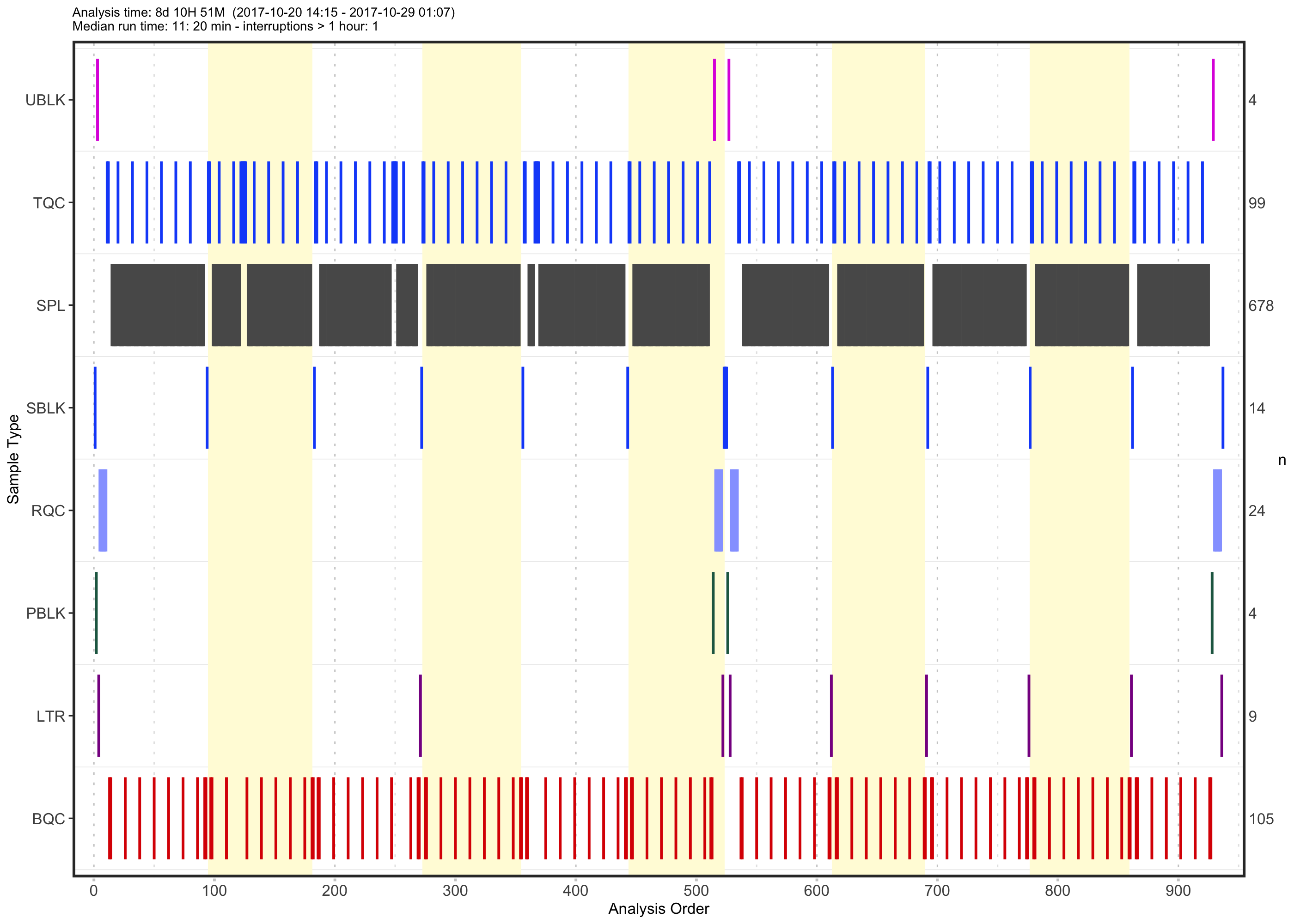
3.2.4 Overall trends and check for possible outliers
To examine overall technical trends and issues affecting most analytes (features), the Relative Log Abundance (RLA) plot is useful (De Livera et al. 2012; Livera et al. 2015). In an RLA plot, each feature is normalized to the across-sample or within-batch median and the resulting values are shown as boxplots for each sample. This visualization helps identify technical problems such as pipetting errors, sample loss, or changes in injection volume or instrument sensitivity.
First, an overview of all analyses (samples) is plotted.
plot_rla_boxplot(
  data = mexp_initial,
  rla_type_batch = c("within"),
  variable = "intensity",
  qc_types = c("BQC", "SPL", "LTR", "TQC", "RQC", "PBLK"),
  filter_data = FALSE,
  #analysis_range = get_batch_boundaries(myexp, batch_indices = c(5,6)),
  y_lim = c(-3, 3), show_timestamp = FALSE, outlier_method = "iqr",
  outlier_k = 1.5, font_base_size = 6, outlier_exclude = FALSE,
  x_gridlines = FALSE, batch_zebra_stripe = FALSE, linewidth = 0.1,
  show_plot = TRUE)
ℹ Found 26 outliers in the 919 shown analyses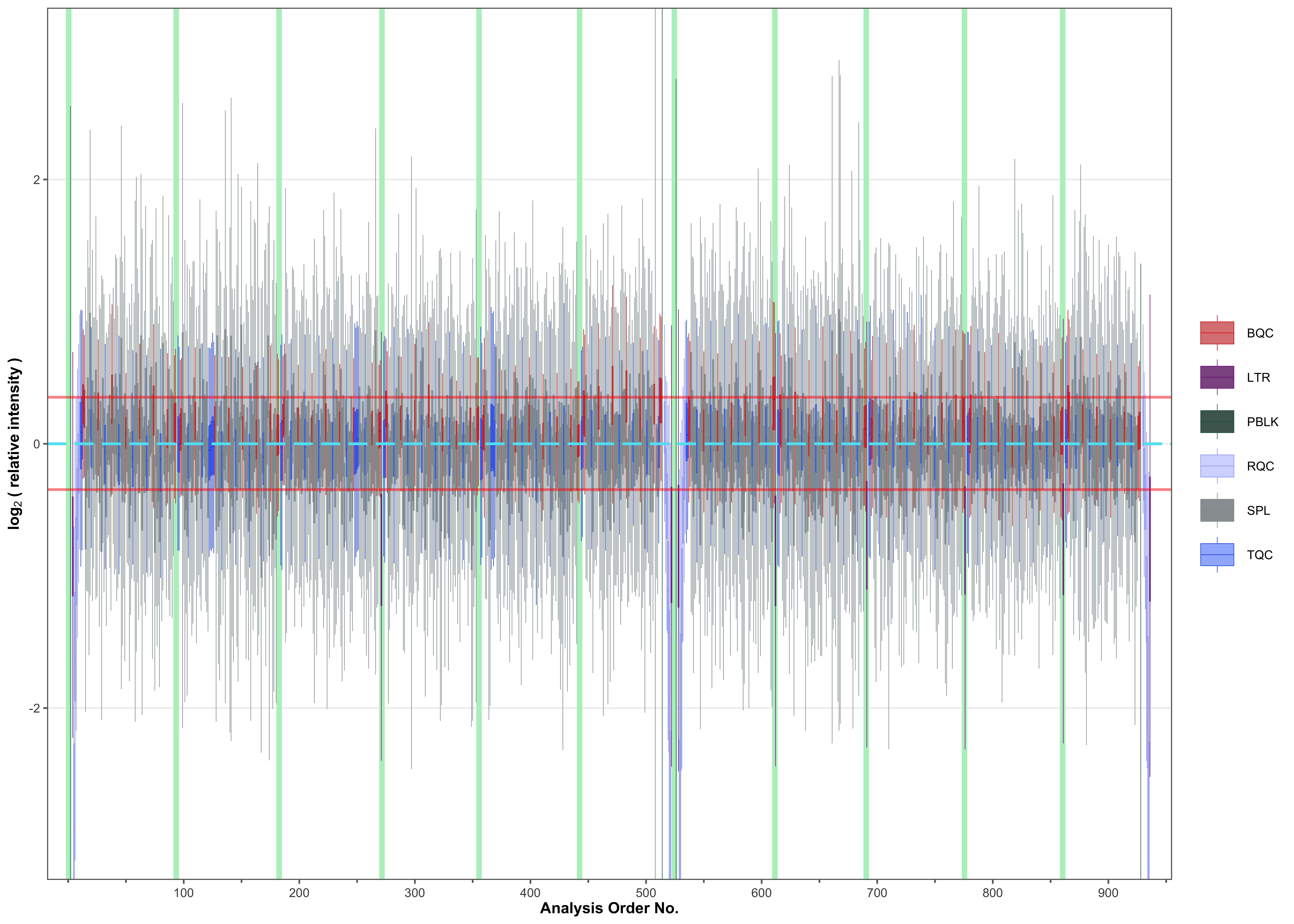
A zoom-in reveals that the endogenous (non-ISTD) features of one QC sample type, the LTRs, have on average approximately half the intensity of the other samples.
# An outlier sample, discussed later, is excluded here for demonstration
# purposes.

mexp_initial_temp <- mexp_initial
mexp_initial_temp <- exclude_analyses(
  mexp_initial_temp,
  analyses = "Longit_batch6_51", clear_existing = TRUE)
✔ 1 analysis was excluded for downstream processing. Please reprocess data.res <- plot_rla_boxplot(
data = mexp_initial_temp,
rla_type_batch = c("across"),
variable = "intensity",
qc_types = c("BQC", "SPL", "LTR", "TQC", "RQC"),
filter_data = FALSE,
exclude_feature_filter = "ISTD",
plot_range = c(595, 696),
y_lim = c(-2, 1.5),
include_istd = FALSE,
include_qualifier = FALSE,
min_feature_intensity = 500, show_timestamp = FALSE,
outlier_method = "iqr", outlier_k = 1.5,
#outlier_k = c(-1, 1),
outlier_exclude = FALSE, x_gridlines = FALSE, batch_zebra_stripe = FALSE,
font_base_size = 6, show_plot = FALSE, linewidth = 0.1)ℹ Found 20 outliers in the 914 shown analysesfig4b <- res$plot
fig4b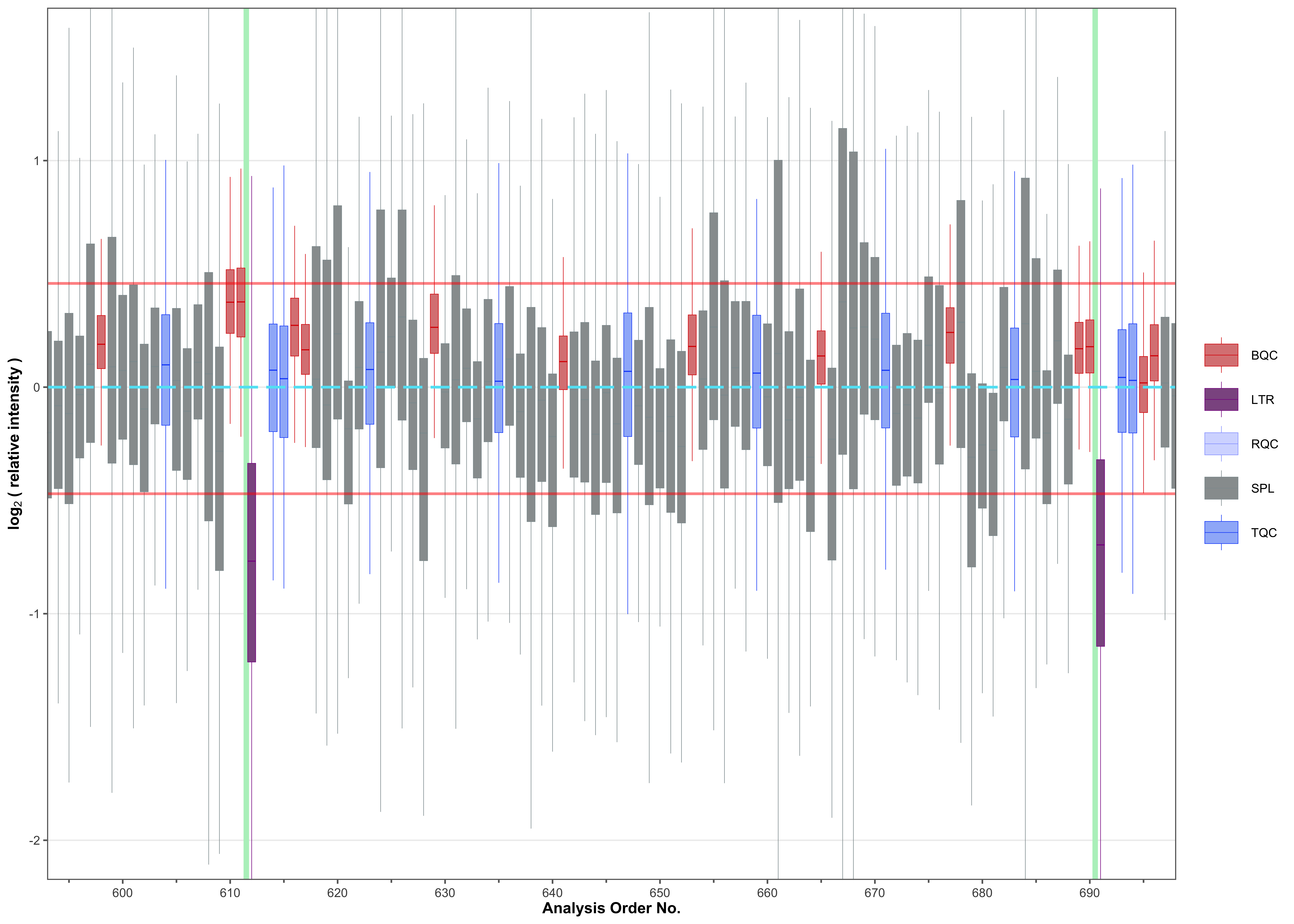
Now we plot the distributions of the ISTDs only. We see that they, too, have approximately half the intensity in the LTR samples compared to the other samples. This may suggest that the measured sample amount was lower for the LTR samples, or that twice the amount of extraction solvent was added, both of which will lead to reduction of all features, including ISTDs.
extfig4b <- plot_rla_boxplot(
  data = mexp_initial,
  rla_type_batch = c("across"),
  variable = "intensity",
  qc_types = c("BQC", "SPL", "LTR", "TQC", "RQC", "PBLK"),
  filter_data = FALSE,
  include_feature_filter = "ISTD",
  plot_range = c(595, 696),
  y_lim = c(-2, 1.5),
  include_istd = TRUE,
  include_qualifier = FALSE,
  min_feature_intensity = 500, show_timestamp = FALSE,
  outlier_method = "iqr", outlier_k = 1.5, outlier_exclude = FALSE,
  x_gridlines = FALSE, batch_zebra_stripe = FALSE, show_plot = FALSE,
  font_base_size = 8, linewidth = 0.2)$plot
ℹ Found 13 outliers in the 919 shown analysesextfig4b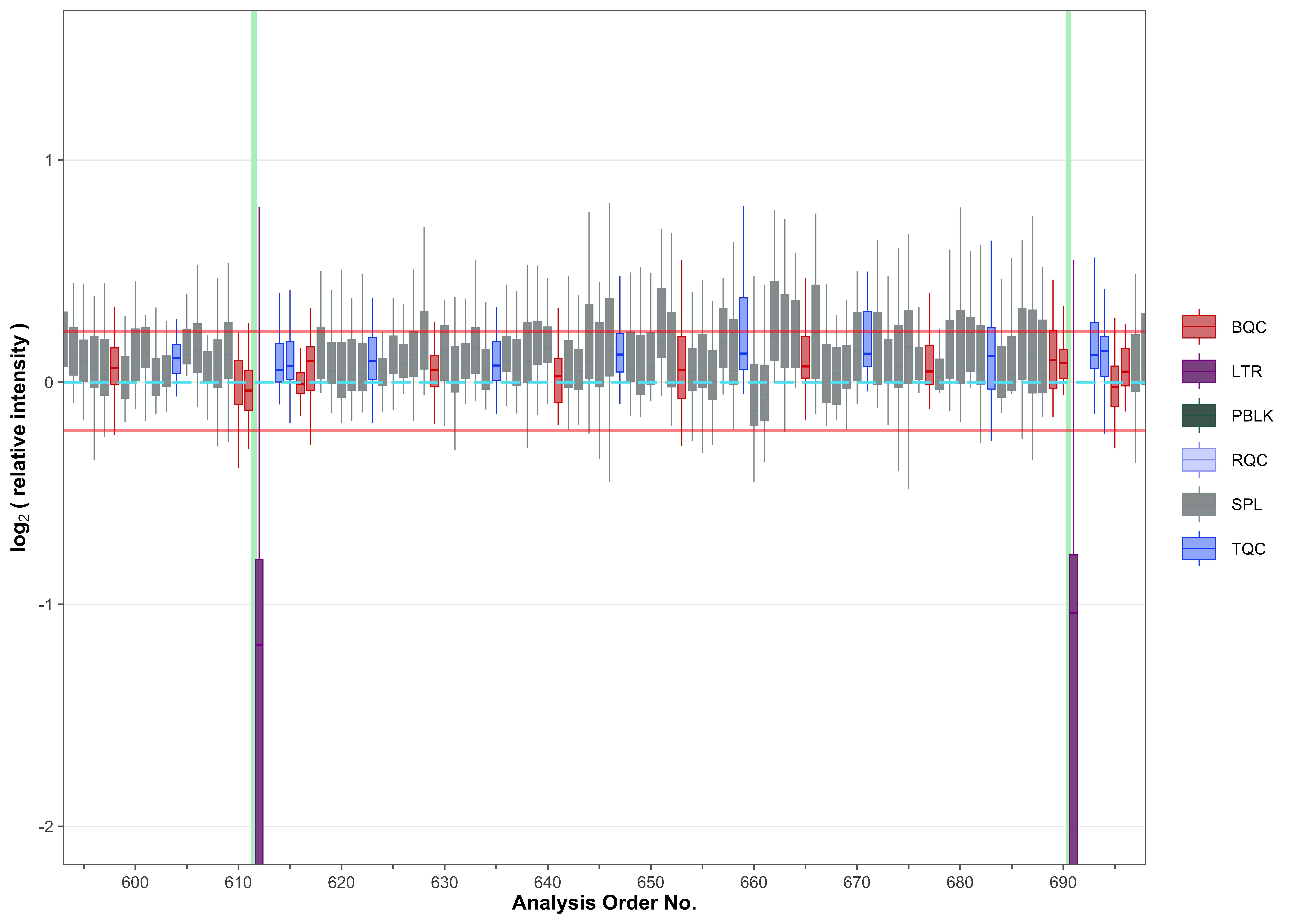
A further, detailed, batch-by-batch inspection revealed that in batch 6, the sample “Longit_batch6_51” at position 464 had markedly lower intensities of non-ISTD features, comparable to those of the blanks.
extfig4c <- plot_rla_boxplot(
  data = mexp_initial,
  rla_type_batch = c("across"),
  variable = "intensity",
  qc_types = c("BQC", "SPL", "LTR", "TQC", "RQC", "PBLK"),
  filter_data = FALSE,
  plot_range = c(430, 522),
  y_lim = c(-10, 1.5),
  include_istd = FALSE,
  exclude_feature_filter = "ISTD",
  include_qualifier = FALSE,
  min_feature_intensity = 500, show_timestamp = FALSE,
  outlier_method = "iqr", outlier_k = 1.5, outlier_exclude = FALSE,
  x_gridlines = FALSE, batch_zebra_stripe = FALSE, font_base_size = 6,
  show_plot = FALSE, linewidth = 0.2,
  legend_position = c(0.3, 0.32), legend_size = 8, strip_text_size = 8)$plot
ℹ Found 20 outliers in the 919 shown analysesextfig4c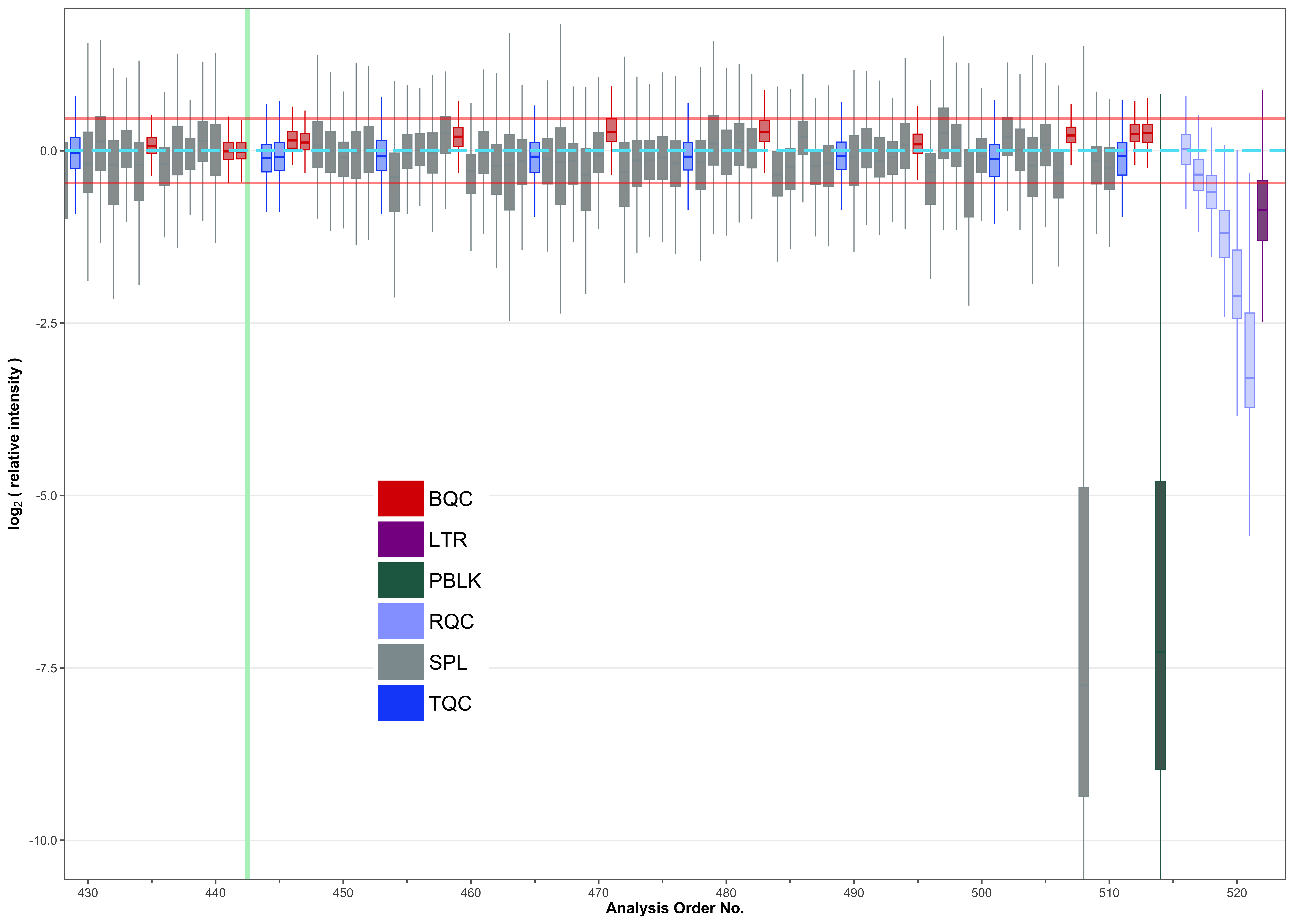
However, the ISTD signals were comparable with other samples. This likely suggests that this study sample was not added to the extraction vial before extraction. The sample will be excluded from further analysis.
mexp_initial_temp2 <- mexp_initial
mexp_initial_temp2@dataset <- mexp_initial_temp2@dataset |> filter(is_istd)

extfig4d <- plot_rla_boxplot(
  data = mexp_initial_temp2,
  rla_type_batch = c("across"),
  variable = "intensity",
  qc_types = c("BQC", "SPL", "LTR", "TQC", "RQC", "PBLK"),
  filter_data = FALSE,
  plot_range = c(430, 522),
  y_lim = c(-10, 1.5),
  include_istd = TRUE,
  include_feature_filter = "ISTD",
  include_qualifier = FALSE,
  min_feature_intensity = 500, show_timestamp = FALSE,
  outlier_method = "iqr", outlier_k = 1.5, outlier_exclude = FALSE,
  x_gridlines = FALSE, batch_zebra_stripe = FALSE, font_base_size = 8,
  show_plot = FALSE, linewidth = 0.2,
  legend_position = c(0.3, 0.32), legend_size = 8, strip_text_size = 8)$plot
ℹ Found 20 outliers in the 919 shown analysesextfig4d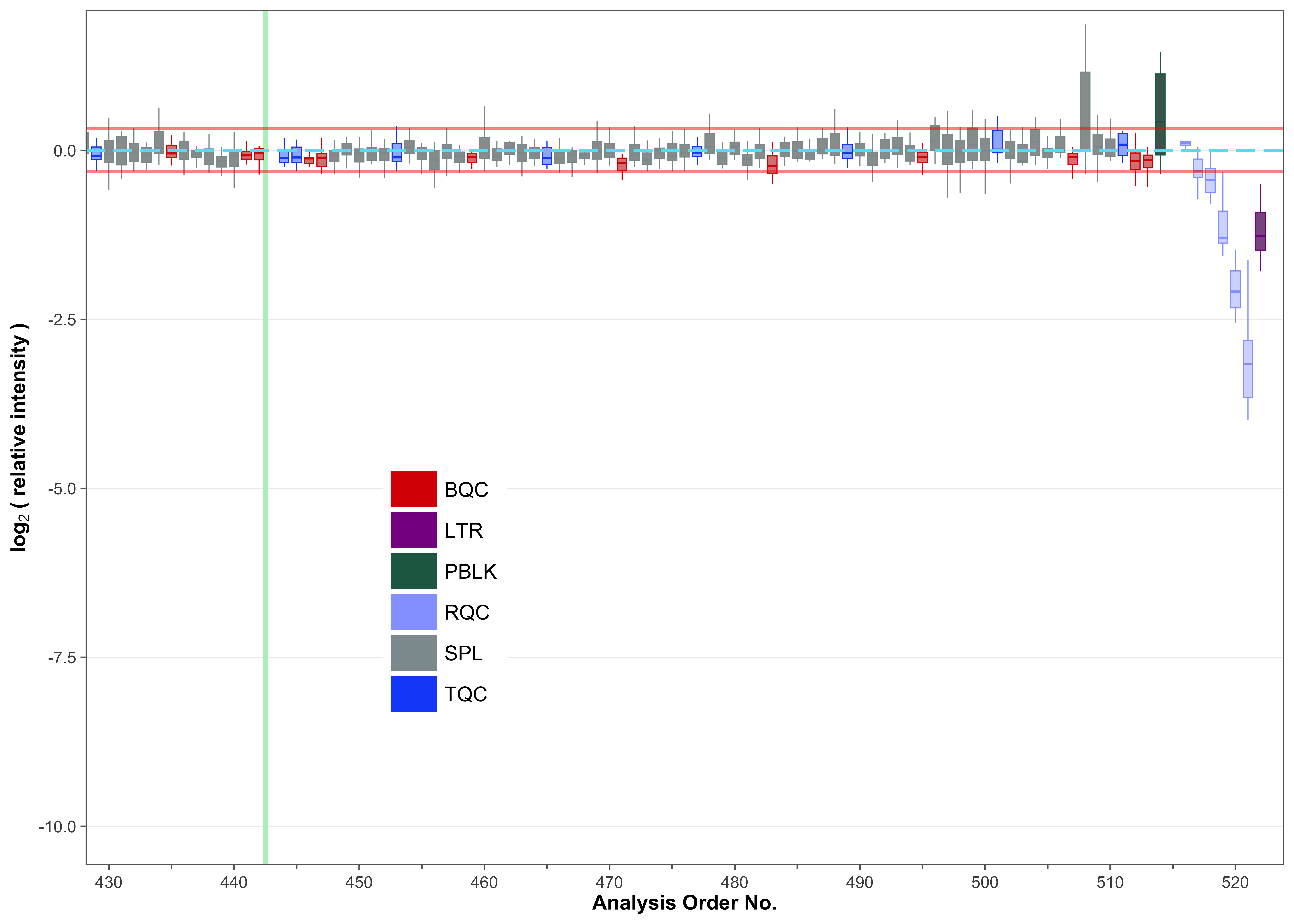
3.3 Peak annotation QC
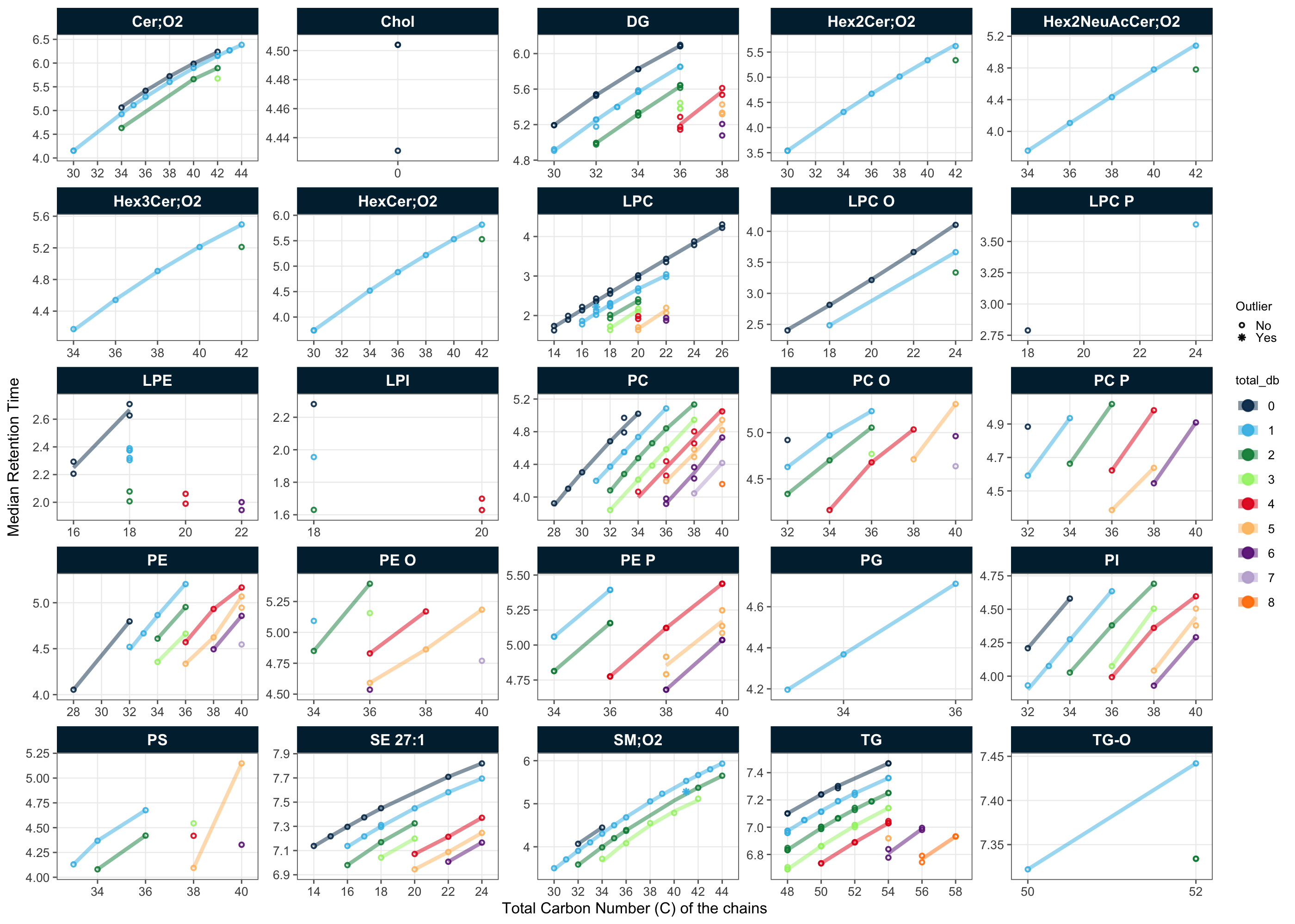
To check for potential peak-picking errors from the integration step (see the section above), the retention time (RT) of the lipid features is plotted against their total carbon number and number of double bonds. Here we apply this plot to the initial integration imported above; the example shown is the PC class. Reviewing these plots across all lipid classes flagged several potential peak-picking errors, notably among the SM, most likely caused by erroneous picking of the isobaric isotopologue peaks of the corresponding PCs. These are corrected further below, where the before/after comparison across all classes is shown. Lipid species that remained flagged as potential misannotations were manually inspected in the chromatograms and compared with an online resource for lipid RTs measured using the same LC-MS method (https://metabolomics.baker.edu.au/method/lipids), and were deemed likely correct.
mexp_initial <- exclude_analyses(
  mexp_initial,
  analyses = "Longit_batch6_51", clear_existing = TRUE)
✔ 1 analysis was excluded for downstream processing. Please reprocess data.mexp_temp <- mexp_initial
mexp_temp@dataset <- mexp_temp@dataset |>
filter(str_detect(feature_id, "^PC \\d"))
fig4c <- plot_rt_vs_chain(
mexp_temp,
qc_types = "SPL",
x_var = "total_c", font_base_size = 6,
legend_position = "right", legend_size = 0.8)ℹ The following features were flagged as potential annotation outliers: PC 30:0 (b), PC 32:1, PC 32:2, PC 38:3 (a)fig4c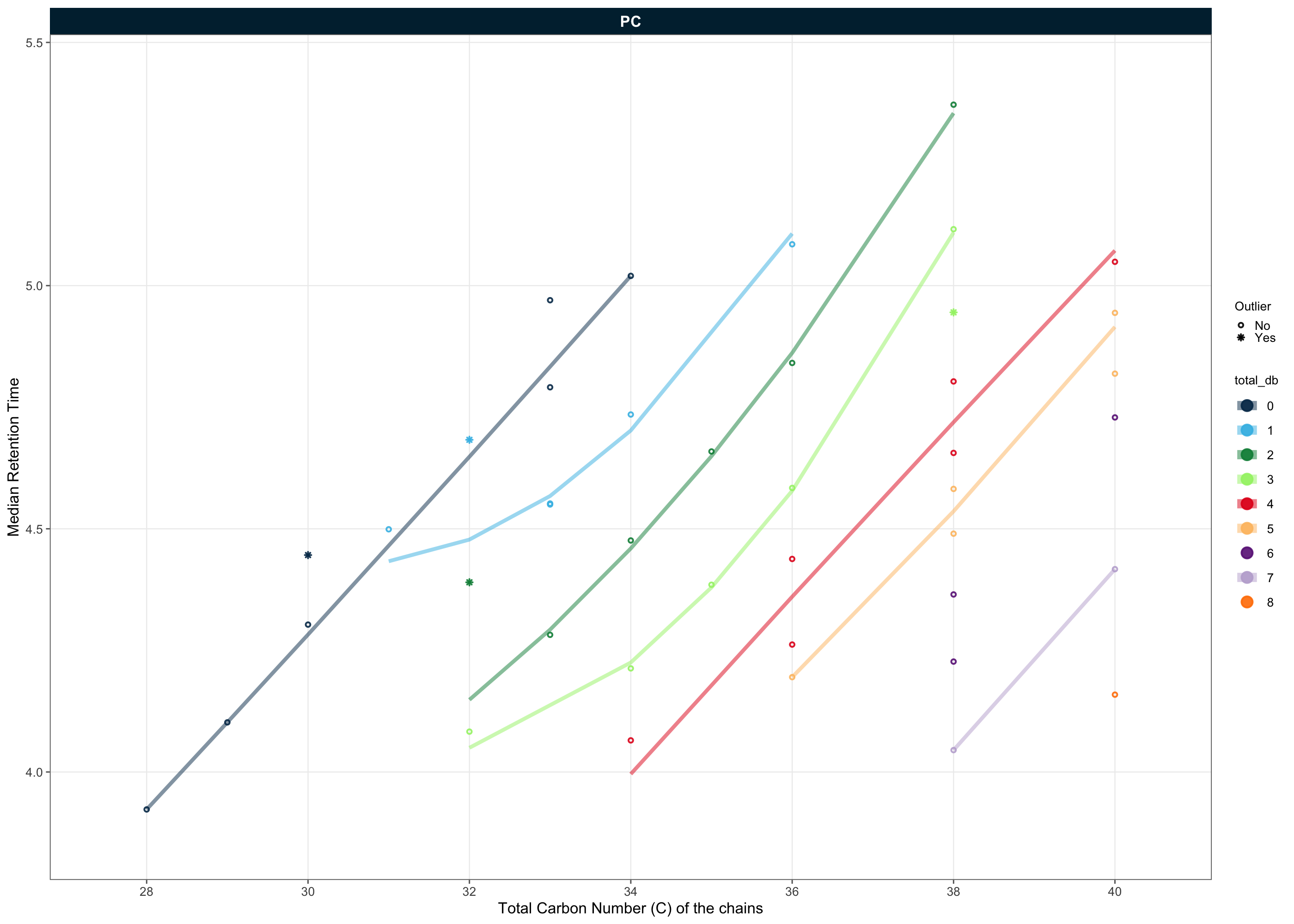
3.4 Feature correlation analysis
As another check for potential peak picking errors, highly correlating features are plotted.
# Exclude the sample identified above as having very low intensities for all
# non-ISTD features.
mexp_initial <- exclude_analyses(
  mexp_initial,
  analyses = "Longit_batch6_51", clear_existing = TRUE)
✔ 1 analysis was excluded for downstream processing. Please reprocess data.fig4d <- plot_feature_correlations(
mexp_initial,
variable = "intensity",
include_feature_filter = c("Cer d18:1/24:0", "Cer d18:0/24:1"),
qc_types = c("SPL", "BQC", "TQC"),
cor_min = 0.1, sort_by_corr = TRUE, return_plots = TRUE,
show_progress = FALSE, log_scale = FALSE, cols_page = 1, rows_page = 1,
font_base_size = 6)[[1]] +
theme(
strip.text = ggplot2::element_text(size = 6),
#aspect.ratio = 0.9,
legend.position = "inside", axis.text = element_text(size = 5),
legend.direction = "vertical",
legend.text = element_text(size = 6 * 0.7),
legend.title = element_text(size = 6 * 0.7),
legend.key.size = unit(6 * 0.7, "pt"),
legend.position.inside = c(0.9, 0.12))ℹ Generating plots (1 page)...fig4d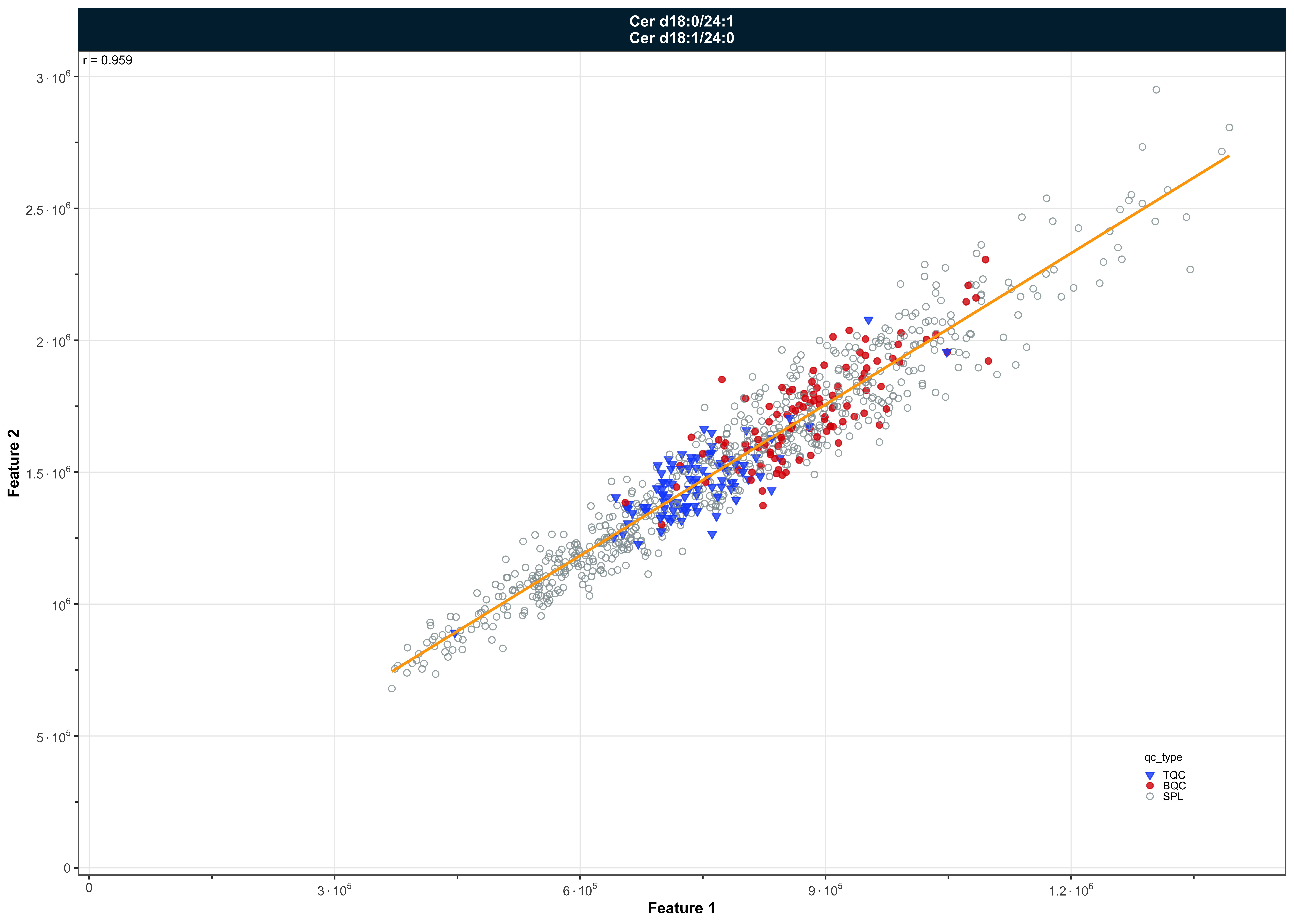
3.5 Fix peak integration and re-import data (V2)
We now went back to the MRMhub-INTEGRATOR workflow and corrected the peak integration errors. The corrected data is available in the file Dataset1_MRMhub-INTEGRATOR_Final.csv. We import this corrected data, which we will use from now on.
mexp <- MRMhubExperiment()
mexp <- import_data_mrmhub(
  mexp,
  "./data/dataset-1/Dataset1_MRMhub-INTEGRATOR_Final.csv")
✔ Imported 937 analyses with 482 features.ℹ feature_area selected as default feature intensity. Modify with `set_intensity_var()`.✔ Analysis metadata associated with 937 analyses.✔ Feature metadata associated with 482 features.Using the same QC plot as above, we now compare the initial integration with the corrected data across all lipid classes. The peak-picking errors, in particular among the SM, appear to have been resolved.
extfig5a <- plot_rt_vs_chain(
  mexp_initial,
  qc_types = "SPL",
  x_var = "total_c", font_base_size = 6,
  legend_position = "right", legend_size = 0.8)
ℹ The following features were flagged as potential annotation outliers: DG 18:1_20:0 [-18:1], DG 14:1_20:0 [-20:0], LPC 17:1 (c), PC 30:0 (b), PC 32:1, PC 32:2, PC 38:3 (a), SM 41:1 (a), SM 40:1, SM 39:1, SM 44:2 M+2, SM 42:2, SM 36:2, SM 36:2 d9 (ISTD), SM 35:2, SM 32:2, SM 38:3|PC 33:1 d7 M+2, SM 34:3, TG 48:0 d5 (ISTD) [-16:0], TG O-51:2 [-18:1]extfig5a
extfig5b <- plot_rt_vs_chain(
mexp,
qc_types = "SPL",
x_var = "total_c", font_base_size = 6,
legend_position = "right", legend_size = 0.8)ℹ The following features were flagged as potential annotation outliers: LPC 17:1 (c), SM 41:1 (a)extfig5b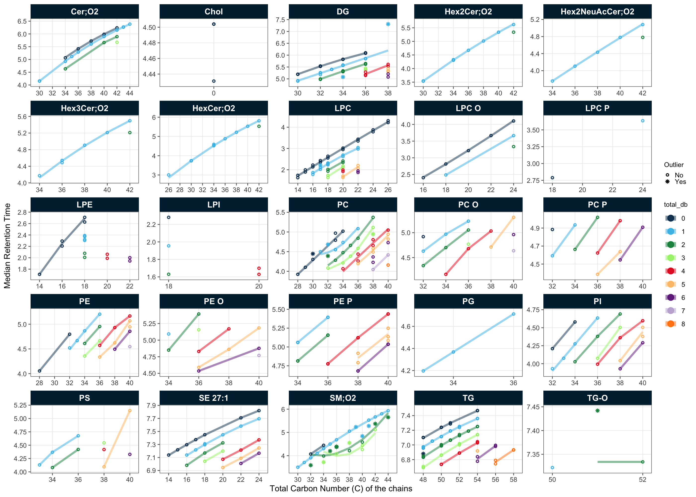
3.6 PCA to check for potential technical outliers
extfig6a <- plot_pca(
  data = mexp,
  variable = "intensity",
  filter_data = FALSE,
  pca_dims = c(1, 2), labels_threshold_mad = 4,
  qc_types = c("SPL", "BQC", "TQC", "LTR"),
  ellipse_variable = "qc_type",
  log_transform = TRUE, point_size = 1, point_alpha = 0.7,
  font_base_size = 8, ellipse_alpha = 0.3,
  include_istd = FALSE,
  show_labels = TRUE, label_font_size = 2, shared_labeltext_hide = NA,
  legend_position = "right", legend_size = 0.7)
! 9 features contained missing or non-numeric values and were exluded.✔ The PCA was calculated based on `feature_intensity` values of 465 features.extfig6a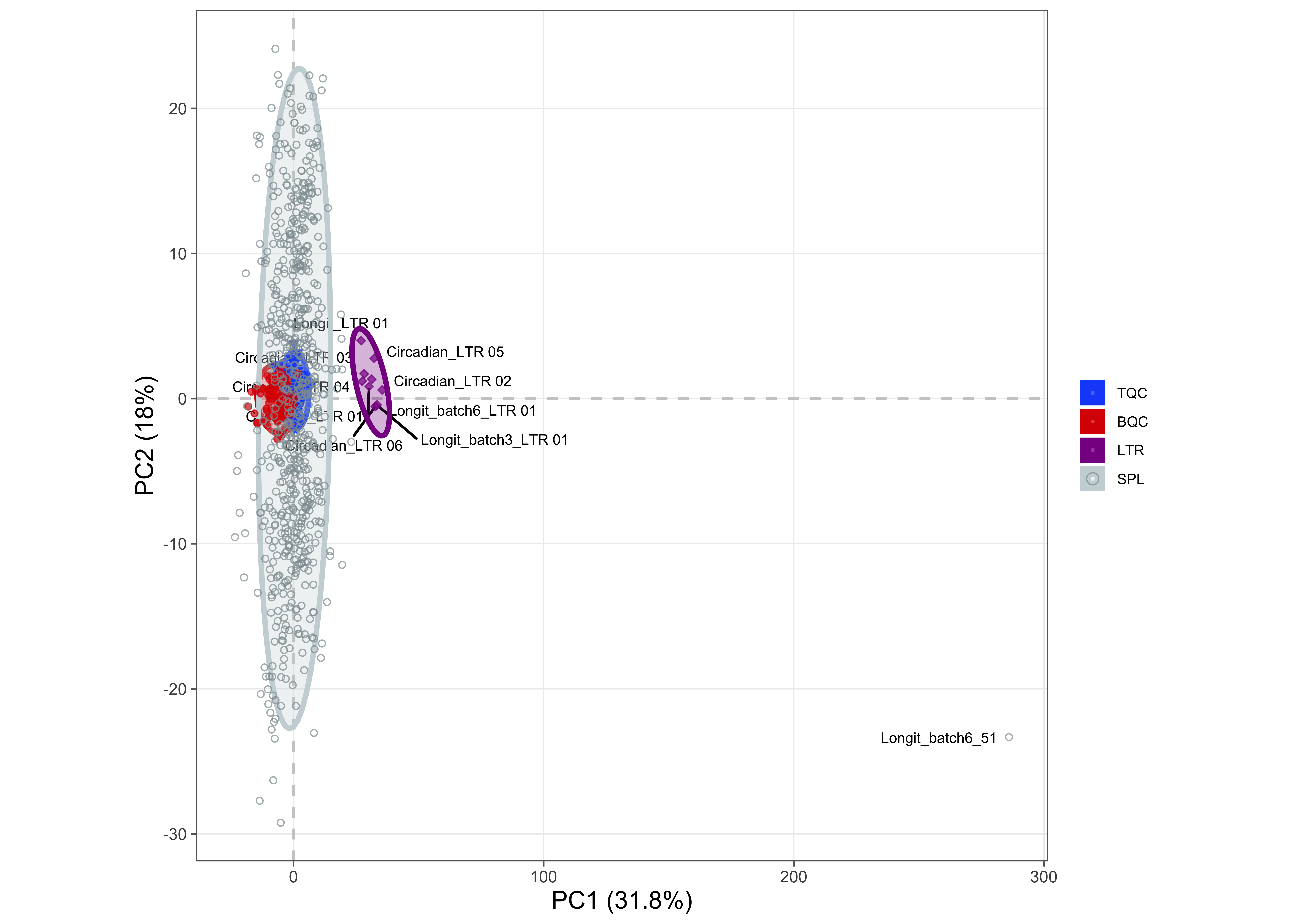
3.7 Exclude outlier analysis/sample and replot PCA
mexp <- exclude_analyses(
  mexp,
  analyses = "Longit_batch6_51", clear_existing = FALSE)
✔ 1 analysis is now excluded for downstream processing. Please reprocess data.fig4e <- plot_pca(
data = mexp,
variable = "intensity",
filter_data = FALSE,
pca_dims = c(1, 2), labels_threshold_mad = 4,
qc_types = c("SPL", "BQC", "TQC"),
ellipse_variable = "qc_type",
log_transform = TRUE, point_size = 1, point_alpha = 0.7,
font_base_size = 6, ellipse_alpha = 0.3,
include_istd = FALSE,
show_labels = FALSE, label_font_size = 2, shared_labeltext_hide = NA,
legend_position = "inside-tr", legend_size = 0.7, legend_bg_alpha = 0.6)! 9 features contained missing or non-numeric values and were exluded.✔ The PCA was calculated based on `feature_intensity` values of 465 features.fig4e
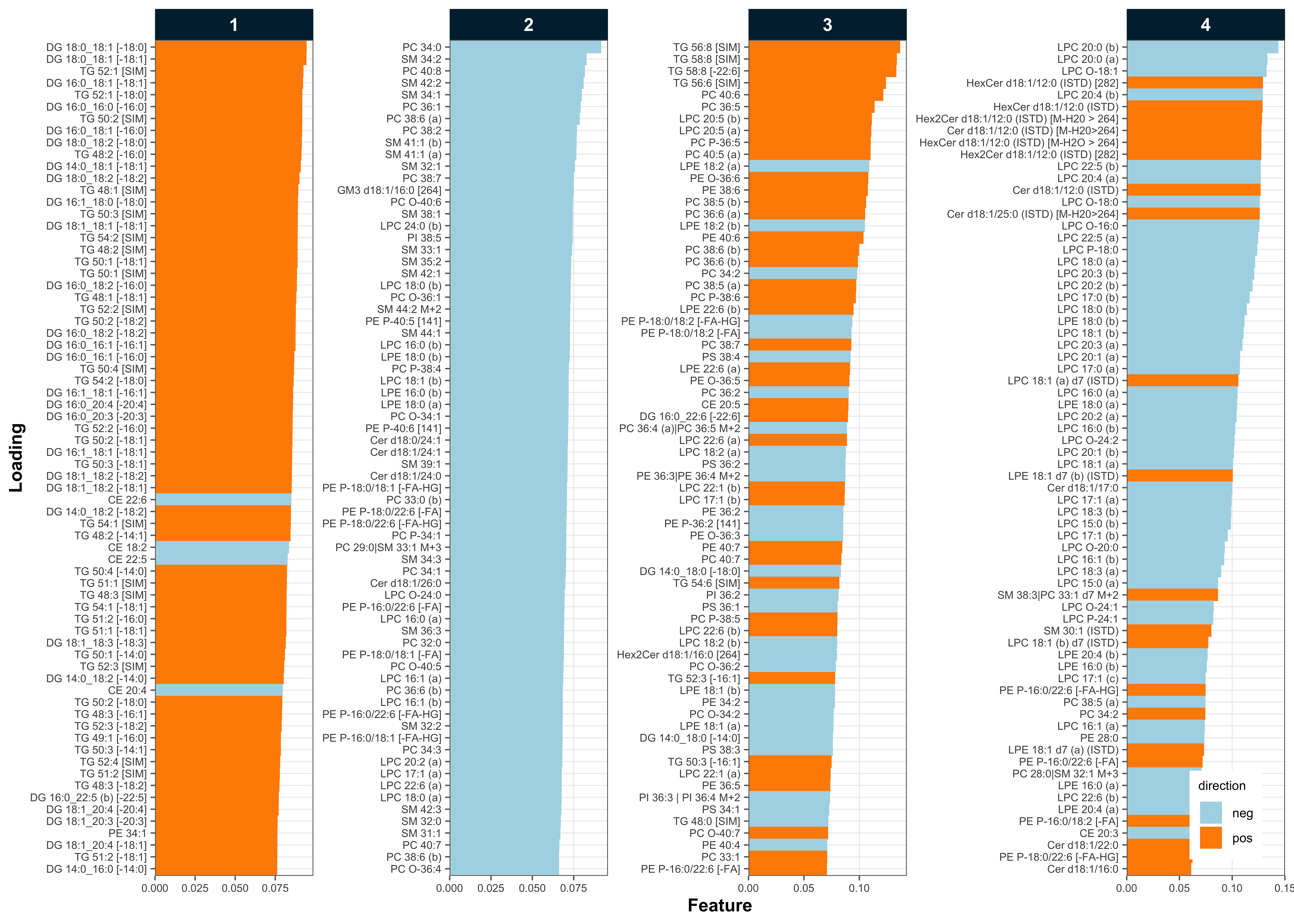
extfig6b <- plot_pca_loading(
data = mexp,
variable = "feature_intensity",
include_istd = FALSE,
pca_dims = c(1, 2, 3, 4), top_n = 70, font_base_size = 7,
#qc_types = c("SPL", "BQC", "TQC", "LTR"),
log_transform = TRUE,
legend_position = "inside-br", legend_size = 0.7)
extfig6b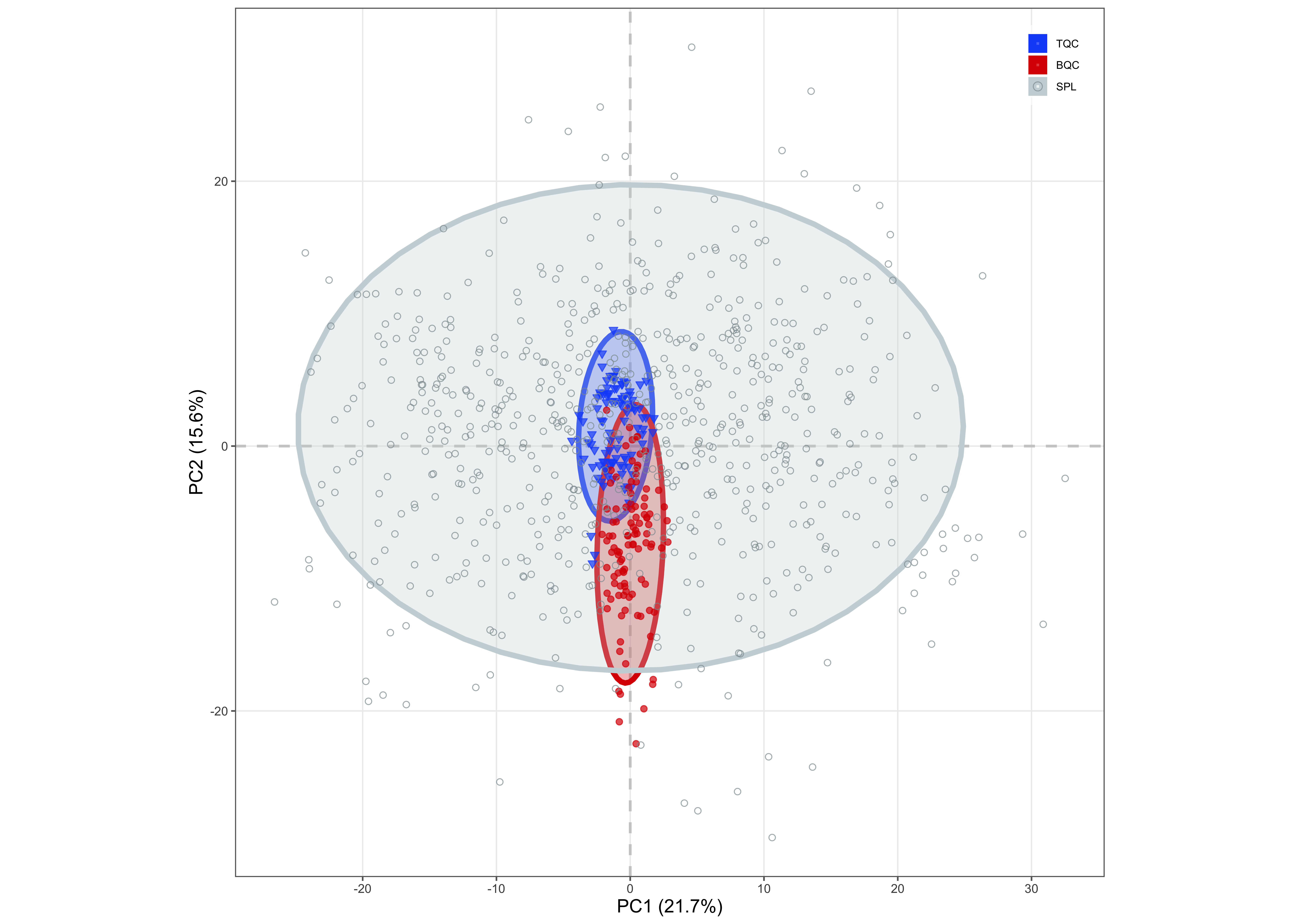
3.8 Importing detailed metadata
Now that the peak integration has been finalized, we import the detailed metadata required for the remaining processing steps; it was not needed for the peak-picking QC and integration curation above, which rely only on the integration results. This metadata describes the analyses/samples, features, internal standards (ISTDs), QC samples, and response curves. We are using the MRMhub MSorganizer template, an Excel template used to collect, organize and pre-validate analysis metadata. Other metadata formats can also be imported, such as CSV files, individual Excel tables, or R data frames.
After metadata import, a summary of the data/metadata integrity validation is returned, e.g. duplicate or missing IDs. Warnings can be ignored (ignore_warnings = TRUE) to proceed with the analysis; errors, such as missing or duplicate IDs, must always be fixed before analysis can proceed.
file_path <- "./data/dataset-1/Dataset1_Metadata.xlsx"
mexp <- import_metadata_msorganiser(mexp, file_path, ignore_warnings = TRUE)
#> Found no errors, 2 warnings, and no notes in the metadata.
#> -----------------------------------------------------------------
#>   Type  Table    Column     Issue                           Count
#> 1 W*    Features feature_id Feature(s) without metadata         5
#> 2 W*    Features feature_id Feature(s) not in analysis data    28
#>
#> -----------------------------------------------------------------
#> E = Error, W = Warning, W* = Suppressed Warning, N = Note
#> -----------------------------------------------------------------
✔ Analysis metadata associated with 937 analyses.✔ Feature metadata associated with 477 features.✔ Internal Standard metadata associated with 18 ISTDs.✔ Response curve metadata associated with 24 annotated analyses.3.9 RunScatter plots
We prepare a run-scatter of the peak areas (intensity) of an example internal standard across all analyses/samples for the assembled manuscript figure.
fig4f <- plot_runscatter(
  mexp,
  variable = "intensity",
  #include_feature_filter = "ISTD",
  qc_types = c("SPL", "BQC", "TQC", "PBLK", "RQC", "SBLK"),
  include_feature_filter = example_species_istd,
  show_reference_lines = TRUE,
  ref_qc_types = "SPL",
  reference_fill_color = "#111111", reference_k_sd = NA, point_size = 1,
  font_base_size = 6, cols_page = 1, rows_page = 1, cap_outliers = TRUE,
  reference_sd_shade = FALSE,
  #batch_zebra_stripe = TRUE,
  output_pdf = FALSE, show_progress = FALSE,
  return_plots = TRUE,
  legend_position = c(0.7, 0.1), legend_size = 0.8)[[1]]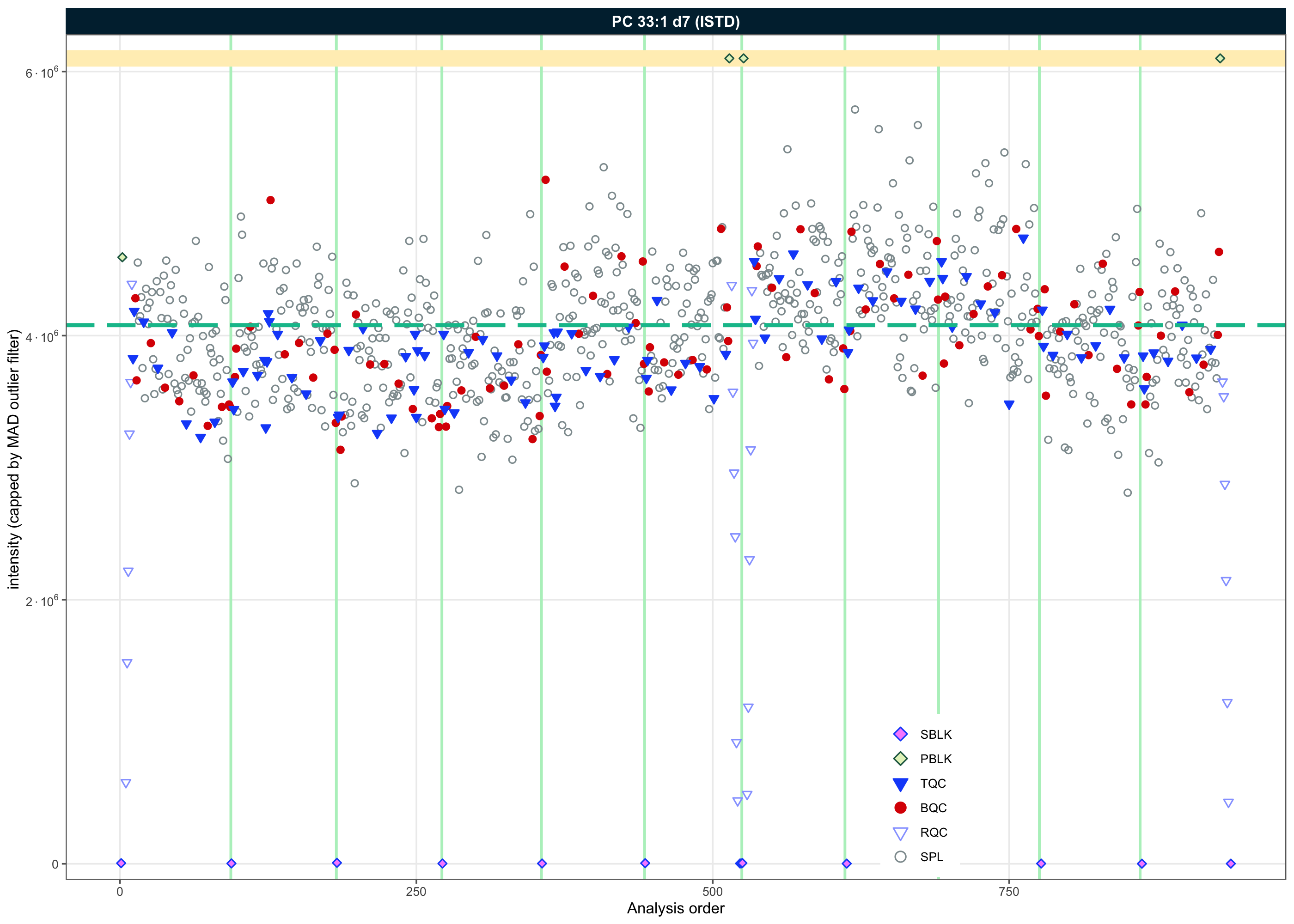
Additionally, we prepare run-scatter plots of all ISTD features (one panel per ISTD) to check for potential issues with individual internal standards; these are collected for the manuscript’s Extended Data figure rather than shown inline here.
extfig7 <- plot_runscatter(
  mexp,
  variable = "intensity",
  include_feature_filter = "ISTD",
  include_qualifier = FALSE,
  qc_types = c("SPL", "BQC", "TQC", "PBLK", "RQC", "SBLK"),
  show_reference_lines = TRUE,
  ref_qc_types = "SPL",
  reference_fill_color = "#111111", reference_k_sd = NA, point_size = .7,
  point_border_width = 0.2, point_alpha = .7, font_base_size = 6,
  cols_page = 4, rows_page = 5, cap_outliers = TRUE,
  reference_sd_shade = FALSE,
  #batch_zebra_stripe = TRUE,
  show_progress = FALSE, output_pdf = FALSE,
  return_plots = TRUE)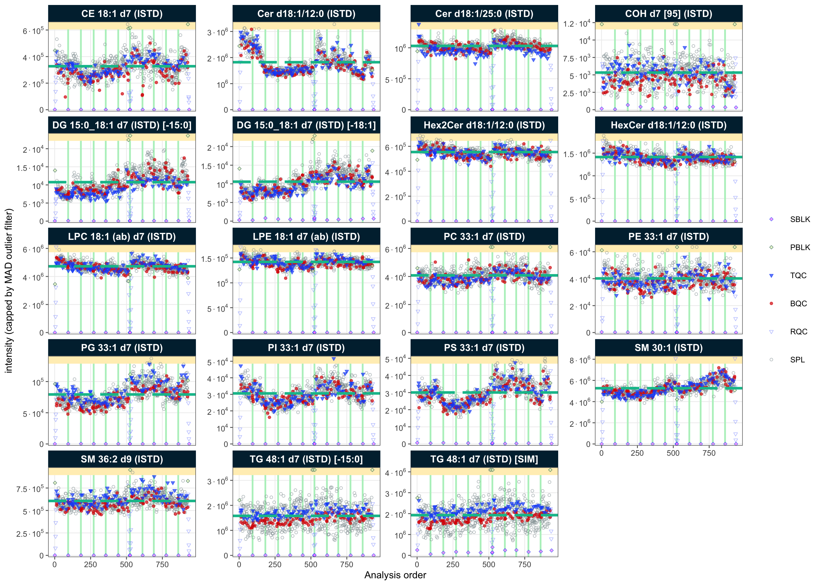
3.10 Matrix effects
To check for potential matrix effects, we plot the peak areas (intensity) of all ISTD features in different QC types.
mexp_temp <- mexp
mexp_temp@dataset <- mexp_temp@dataset |>
  filter(
    !str_detect(feature_id, "DG 15:0\\_18:1 d7 \\(ISTD\\) \\[\\-15:0\\]"))

fig4g <- plot_matrixeffects(
  mexp_temp,
  variable = "intensity",
  y_lim = c(0, 250), point_alpha = 0.55, box_alpha = 0.3, point_size = 0.1,
  box_linewidth = 0.3, font_base_size = 6,
  include_feature_filter = "P[CIE]|DG|TG|Cer|CE",
  min_median_value = 3000)

fig4g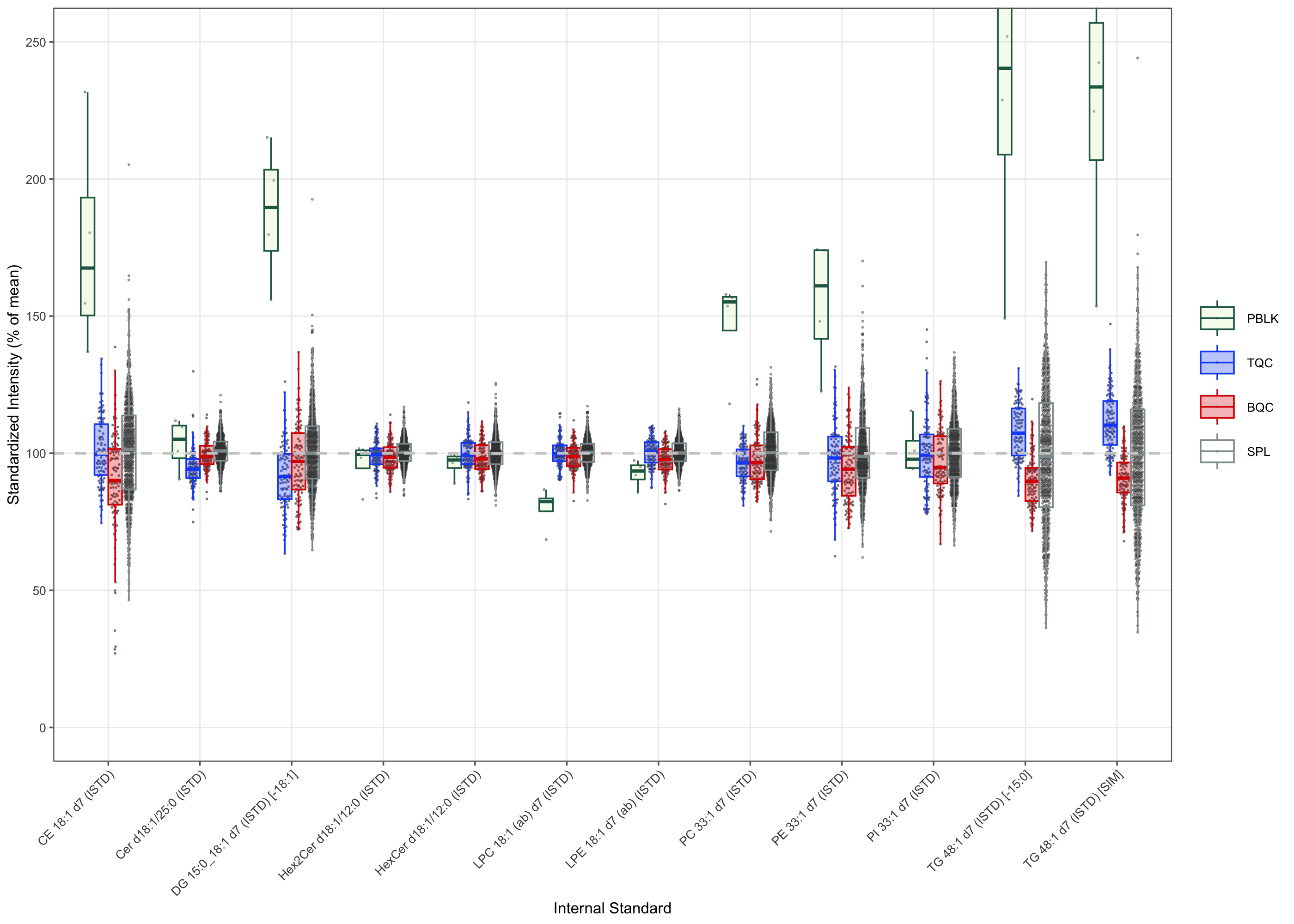
3.11 Normalization and Quantification
The raw peak areas were first normalized by their corresponding internal standard (ISTD), as defined in the feature metadata. Concentrations were then calculated from the spiked-in ISTD amounts and the sample amounts, both also defined in the metadata.
mexp <- normalize_by_istd(mexp)! Interfering features defined in metadata, but no correction was applied. Use `correct_custom_interferences()` to correct.✔ 446 features normalized with 17 ISTDs in 937 analyses.mexp <- quantify_by_istd(mexp)✔ 449 feature concentrations calculated based on 28 ISTDs and sample amounts of 937 analyses.✔ Concentrations are given in μmol/L.3.12 Drift and Batch Correction
After normalization, the feature concentrations were corrected for signal drift within each batch and then re-aligned across batches. Drift was estimated by Gaussian-kernel smoothing over the study samples (ref_qc_types = "SPL"), which most directly reflect the drift affecting the study samples themselves. kernel_size = 20 sets the number of neighbouring samples over which the trend is smoothed, and outlier_ksd = 3 excludes points lying more than three standard deviations from the local trend so that individual outliers do not distort it. The batches were then aligned by sample-based median centering.
mexp <- correct_drift_gaussiankernel(
  mexp,
  variable = "conc",
  ref_qc_types = "SPL",
  batch_wise = TRUE, kernel_size = 20, outlier_filter = TRUE,
  outlier_ksd = 3, recalc_trend_after = TRUE, show_progress = FALSE)
! 7 feature(s) contain one or more zero or negative `conc` values. Verify your data or use `log_transform_internal = FALSE`.! 3 features showed no variation in the study sample's original values across analyses. ! 3 features have invalid values after smoothing. NA will be be returned for all values of these faetures. Set `use_original_if_fail = FALSE to return orginal values..! Smoothing failed for 3 feature(s) in all batches. Please check data, metadata, and fit parameters.! Smoothing failed for 3 feature(s) in at least one batch: COH [161], PG 36:2 and SM 40:2. Please check data, metadata and fit parameters.✔ Drift correction was applied to 446 of 449 features (batch-wise).ℹ The median per-feature CV change of all features in study samples was -0.52% (range: -7.93% to 1.56%; a positive value means the CV increased). The median CV across all features across batches decreased from 38.93% to 38.22%.mexp <- correct_batch_centering(
mexp,
ref_qc_types = "SPL",
log_transform_internal = FALSE,
variable = "conc")! Adding batch correction on top of `conc` drift-correction.✔ Batch median-centering of 11 batches was applied to drift-corrected concentrations of all 477 features.ℹ The median per-feature CV change of all features in study samples was -0.91% (range: -30.20% to 50.80%; a positive value means the CV increased). The median CV across all features decreased from 39.99% to 38.45%.3.13 Concentration run-scatter before and after correction
To visualize the effect of the drift and batch correction, the concentration of an example feature is plotted against the injection order after correction (conc), shown below. The within-batch drift and between-batch offsets present in the raw concentrations (conc_raw) are largely removed after correction; the raw and corrected run-scatters are shown side by side in the assembled manuscript figure.
fig5c <- plot_runscatter(
  mexp,
  variable = "conc_raw",
  #include_feature_filter = "ISTD",
  qc_types = c("SPL", "BQC", "TQC", "LTR"),
  include_feature_filter = example_species,
  #y_min = 0.00,
  #y_max = 0.15,
  #plot_range = c(0, 910),
  show_reference_lines = TRUE,
  ref_qc_types = "SPL",
  reference_fill_color = "#b83c3cff", reference_line_color = "#37c2f0ff",
  reference_k_sd = NA, show_trend = TRUE, point_size = 1,
  font_base_size = 6, cols_page = 1, rows_page = 1, cap_outliers = FALSE,
  reference_sd_shade = FALSE,
  #batch_zebra_stripe = TRUE,
  show_progress = FALSE, output_pdf = FALSE,
  return_plots = TRUE,
  legend_position = c(0.7, 0.1), legend_size = 0.8)[[1]]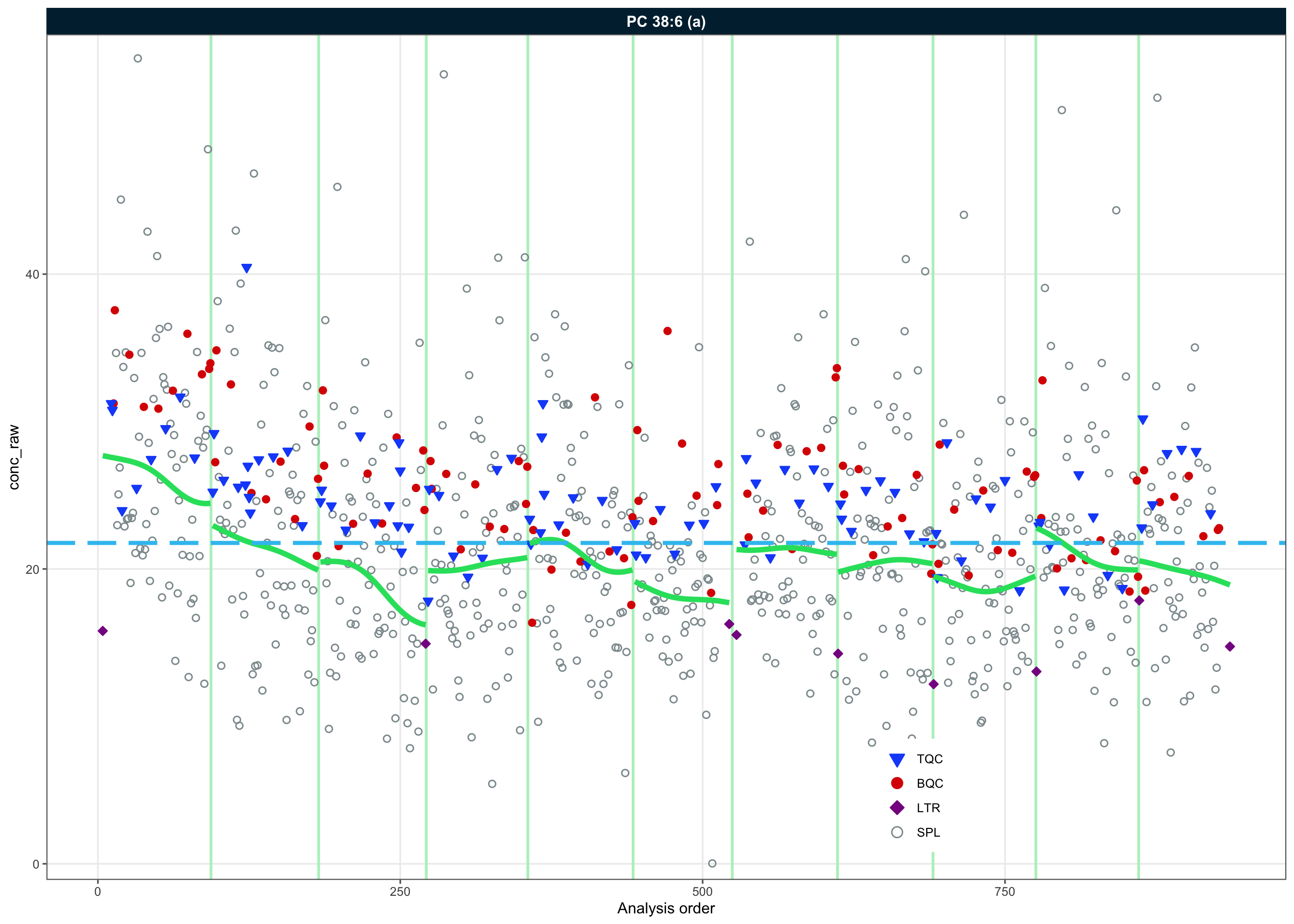
fig5d <- plot_runscatter(
  mexp,
  variable = "conc",
  #include_feature_filter = "ISTD",
  qc_types = c("SPL", "BQC", "TQC", "LTR"),
  include_feature_filter = example_species,
  #y_min = 0.00,
  #y_max = 0.9,
  #plot_range = c(0, 910),
  show_reference_lines = FALSE,
  ref_qc_types = "SPL",
  reference_fill_color = "#111111", reference_line_color = "#37c2f0ff",
  reference_k_sd = NA, show_trend = TRUE, point_size = 1,
  font_base_size = 6, cols_page = 1, rows_page = 1, cap_outliers = FALSE,
  reference_sd_shade = FALSE,
  #batch_zebra_stripe = TRUE,
  show_progress = FALSE, output_pdf = FALSE,
  return_plots = TRUE,
  legend_position = c(0.7, 0.1), legend_size = 0.8)[[1]]

fig5d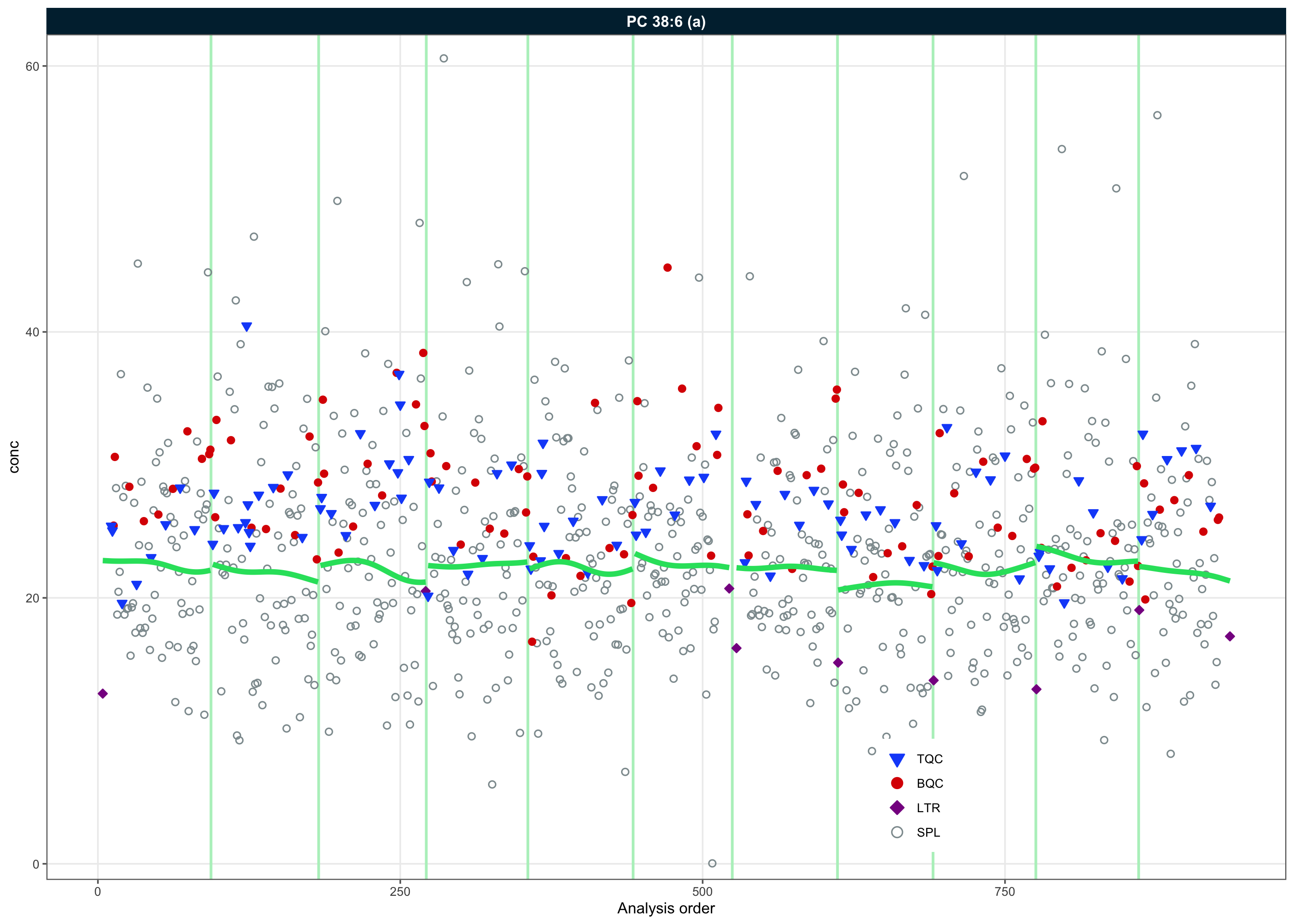
3.14 Normalization and Correction QC
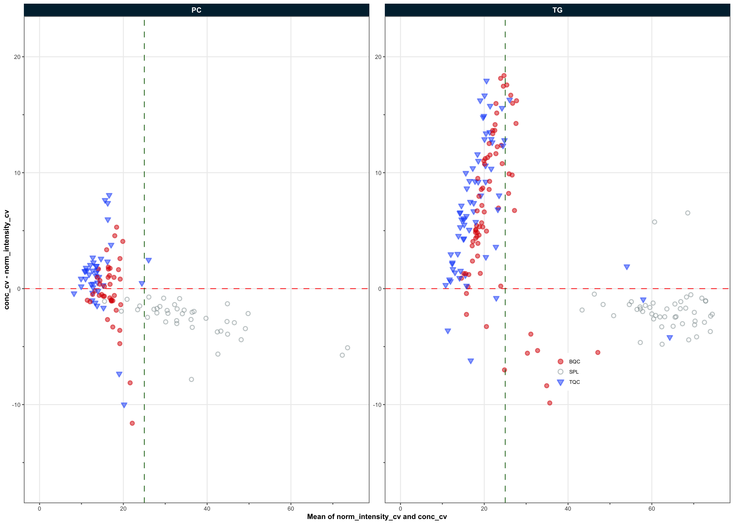
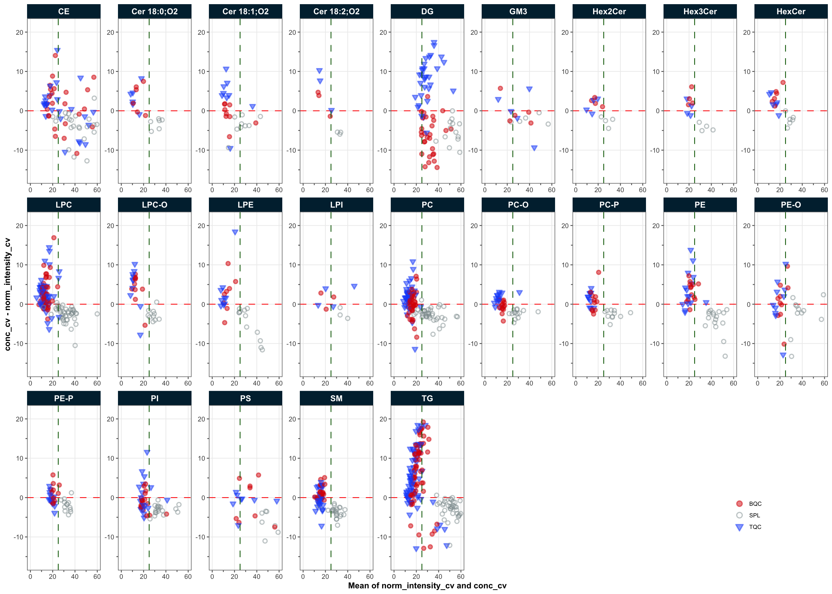
To check whether each processing step reduced technical variability, the per-feature coefficient of variation (CV) is compared before and after the step, as the change in CV per lipid class. The first two plots show the effect of ISTD normalization and of quantification for the PC and TG classes; the following plots repeat this across all classes.
mexp_t1 <- calc_qc_metrics(
  mexp,
  use_robust_cv = TRUE, use_batch_medians = FALSE)
✔ QC metrics calculated for 477 features across 7 sample types, including normalized-intensity, concentration, and response-curve statistics.mexp_t1@metrics_qc <- mexp_t1@metrics_qc |>
dplyr::filter(str_detect(feature_class, "^PC$|TG$"))
mexp_t2 <- calc_qc_metrics(mexp)✔ QC metrics calculated for 477 features across 7 sample types, including normalized-intensity, concentration, and response-curve statistics.mexp_t2@metrics_qc <- mexp_t2@metrics_qc |>
dplyr::filter(str_detect(feature_class, "^PC$|TG$"))
fig5a <- plot_normalization_qc(
plot_type = "diff",
data = mexp_t1,
before_norm_var = "intensity",
after_norm_var = "norm_intensity",
y_lim = c(-15, 20), x_lim = c(0, 75),
qc_types = c("TQC", "BQC", "SPL"),
cols_page = 3, font_base_size = 5, point_size = 1,
facet_by_class = TRUE,
include_qualifier = FALSE,
legend_position = c(0.77, 0.27), legend_size = 0.7)
fig5b <- plot_normalization_qc(
data = mexp_t2,
plot_type = "diff",
before_norm_var = "norm_intensity",
after_norm_var = "conc",
y_lim = c(-15, 20), x_lim = c(0, 75),
qc_types = c("TQC", "BQC", "SPL"),
cols_page = 2,
facet_by_class = TRUE,
font_base_size = 5, point_size = 1,
include_qualifier = FALSE,
legend_position = c(0.77, 0.27), legend_size = 0.7)
fig5a
fig5b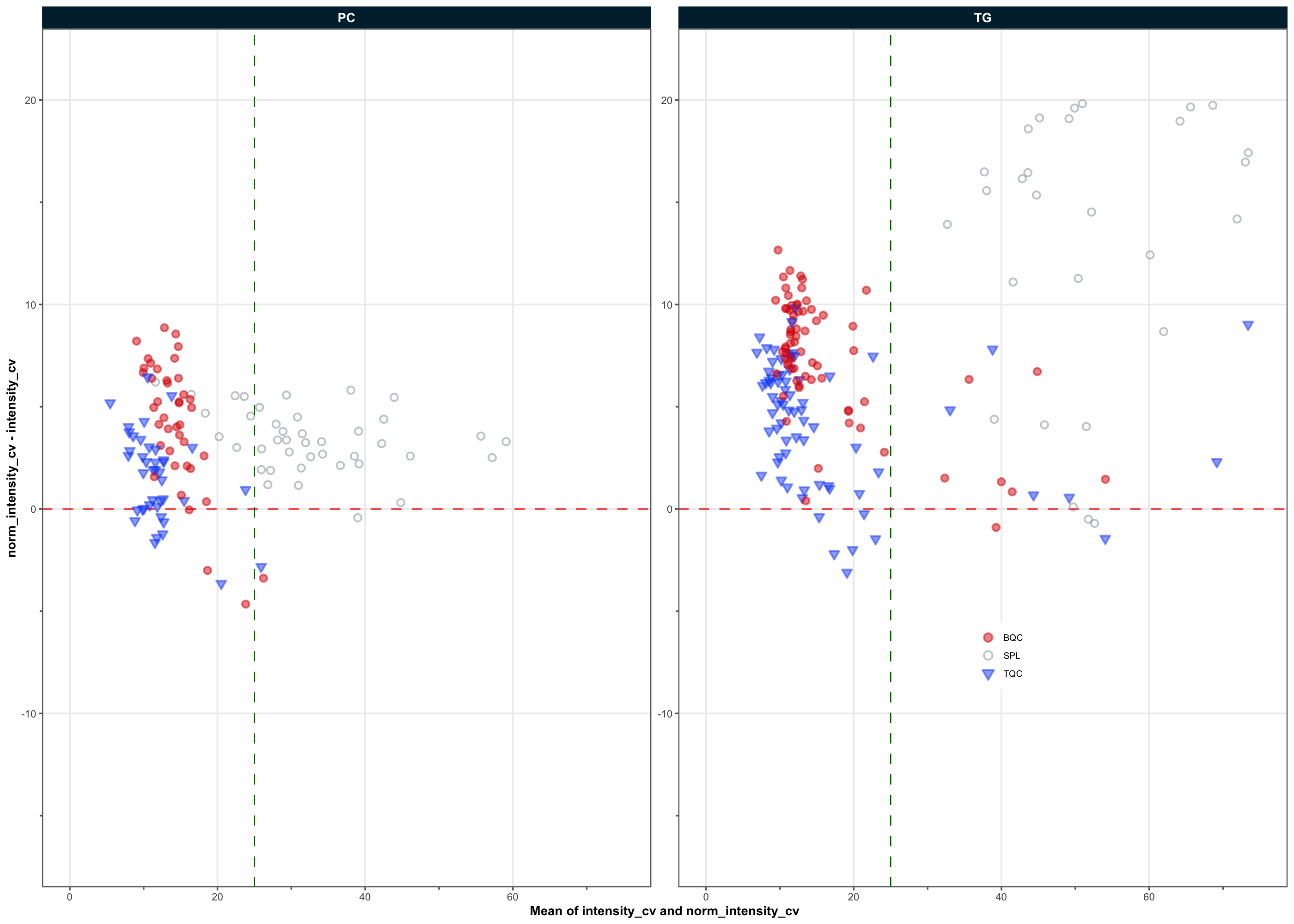
mexp_temp <- calc_qc_metrics(
  mexp,
  use_robust_cv = TRUE, use_batch_medians = FALSE)
✔ QC metrics calculated for 477 features across 7 sample types, including normalized-intensity, concentration, and response-curve statistics.mexp_temp@metrics_qc <- mexp_temp@metrics_qc |>
dplyr::filter(!str_detect(feature_id, "^TG O|COH|PG"))
extfig8a <- plot_normalization_qc(
data = mexp_temp,
before_norm_var = "intensity",
after_norm_var = "norm_intensity",
plot_type = "diff",
y_lim = c(-15, 20), x_lim = c(0, 60),
qc_types = c("TQC", "BQC", "SPL"),
cols_page = 9, font_base_size = 5, point_size = 0.85,
facet_by_class = TRUE,
include_qualifier = FALSE,
legend_position = c(0.9, 0.10), legend_size = 0.7)
extfig8a
extfig8b <- plot_normalization_qc(
data = mexp_temp,
before_norm_var = "norm_intensity",
after_norm_var = "conc",
plot_type = "diff",
y_lim = c(-15, 20), x_lim = c(0, 60),
qc_types = c("TQC", "BQC", "SPL"),
cols_page = 9, font_base_size = 5, point_size = 0.85,
facet_by_class = TRUE,
include_qualifier = FALSE,
legend_position = c(0.9, 0.10), legend_size = 0.7)
extfig8b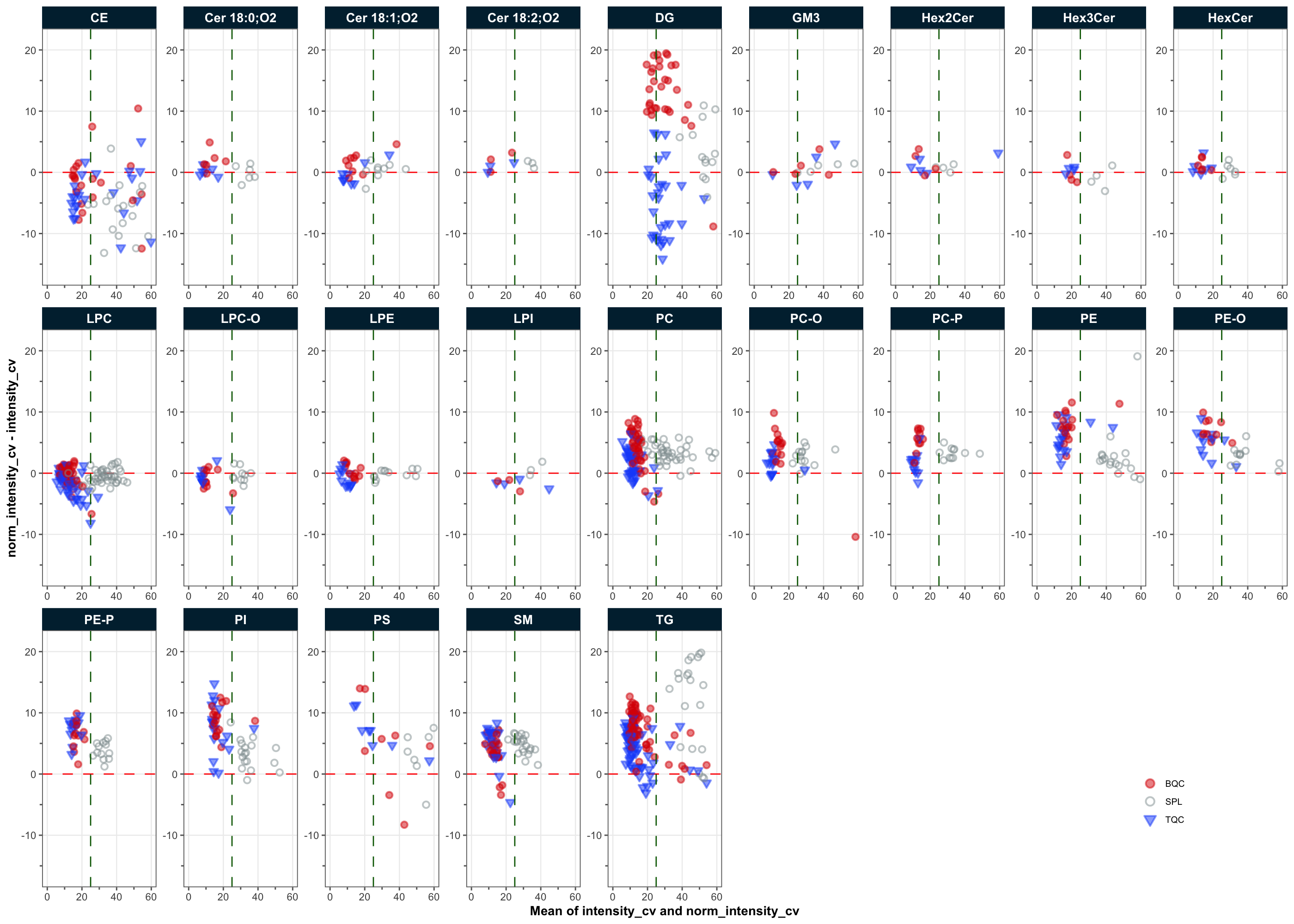
As an alternative to the Gaussian-kernel drift correction used above, a cubic-spline drift correction is shown below. Here the batch QC samples (ref_qc_types = "BQC") are used as the drift reference, as the spline is fitted through the repeatedly measured BQCs rather than smoothed over the study samples.
mexp_spline <- correct_drift_cubicspline(
  mexp,
  variable = "conc",
  ref_qc_types = "BQC",
  batch_wise = TRUE, lambda = 0.5, cv = TRUE, recalc_trend_after = TRUE,
  replace_previous = TRUE)
! Replacing previous `conc` drift and batch corrections...! 7 feature(s) contain one or more zero or negative `conc` values. Verify your data or use `log_transform_internal = FALSE`.! 3 features showed no variation in the study sample's original values across analyses. ! 4 features have invalid values after smoothing. NA will be be returned for all values of these faetures. Set `use_original_if_fail = FALSE to return orginal values..! Smoothing failed for 4 feature(s) in all batches. Please check data, metadata, and fit parameters.! Smoothing failed for 6 feature(s) in at least one batch: CE 15:0, COH [161], LPI 18:0, PC O-34:4, PG 36:2 and SM 40:2. Please check data, metadata and fit parameters.✔ Drift correction was applied to 445 of 449 features (batch-wise).ℹ The median per-feature CV change of all features in study samples was 0.08% (range: -3.49% to 14.38%; a positive value means the CV increased). The median CV across all features across batches decreased from 38.93% to 38.76%.mexp_spline <- correct_batch_centering(
mexp_spline,
ref_qc_types = "BQC",
variable = "conc")! Adding batch correction on top of `conc` drift-correction.✔ Batch median-centering of 11 batches was applied to drift-corrected concentrations of all 477 features.ℹ The median per-feature CV change of all features in study samples was 0.15% (range: -28.20% to 121.90%; a positive value means the CV increased). The median CV across all features increased from 40.78% to 40.89%.mexp_spline <- calc_qc_metrics(
mexp_spline,
use_robust_cv = TRUE, use_batch_medians = FALSE)✔ QC metrics calculated for 477 features across 7 sample types, including normalized-intensity, concentration, and response-curve statistics.mexp_spline@metrics_qc <- mexp_spline@metrics_qc |>
dplyr::filter(!str_detect(feature_id, "^TG O|COH|PG"))
extfig8c <- plot_normalization_qc(
data = mexp_spline,
plot_type = "diff",
before_norm_var = "norm_intensity",
after_norm_var = "conc",
y_lim = c(-20, 20), x_lim = c(0, 60),
qc_types = c("TQC", "BQC", "SPL"),
cols_page = 9, font_base_size = 5, cv_threshold_value = 25,
point_size = 0.85,
facet_by_class = TRUE,
include_qualifier = FALSE,
legend_position = c(0.9, 0.10), legend_size = 0.7)
extfig8c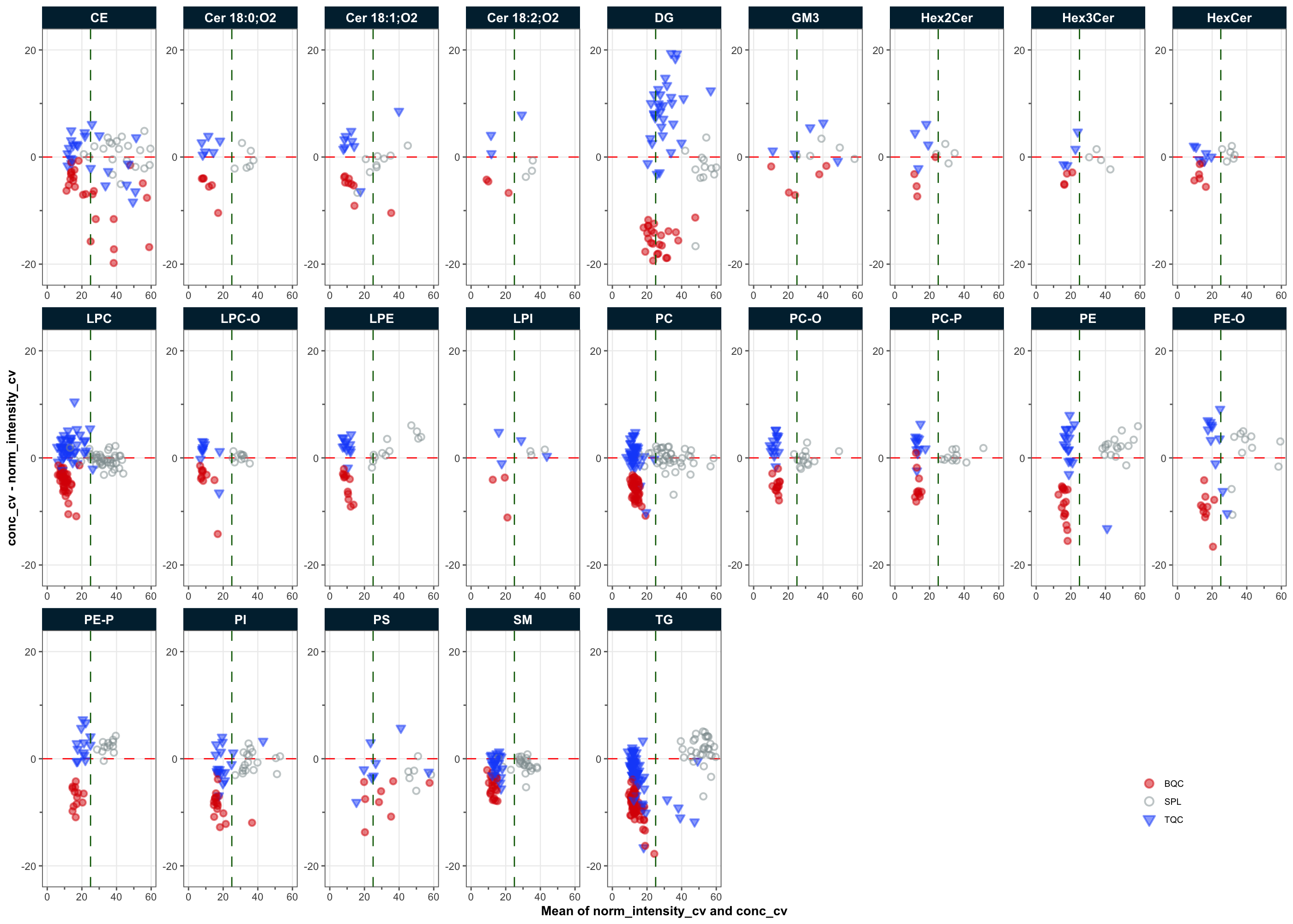
3.15 Technical variability versus intensity
Comparing technical variability of features with their abundances can reveal the intensity threshold at which feature signals exhibit increased noise and variability. This information can be applied during peak picking to set appropriate intensity thresholds for feature detection and to reduce time spent on integrating low abundant features.
mexp <- calc_qc_metrics(
  mexp,
  use_robust_cv = FALSE, use_batch_medians = TRUE)
! %CV not computed for 11270 feature×QC-type×variable combinations with fewer than 3 replicates (LTR: 11267, TQC: 3).✔ QC metrics calculated for 477 features across 7 sample types, including normalized-intensity, concentration, and response-curve statistics.fig5e <- plot_qcmetrics_comparison(
mexp,
plot_type = "scatter",
y_shared = FALSE,
x_variable = "intensity_median_bqc",
y_variable = "intensity_cv_bqc",
log_scale = FALSE, equality_line = FALSE,
facet_by_class = FALSE,
point_size = 1.1, font_base_size = 6,
#x_lim = c(0, Inf),
y_lim = c(0, 100), legend_position = "none") +
ggplot2::geom_smooth(method = "loess", se = FALSE, span = 0.75) +
geom_hline(yintercept = 20, linetype = "dashed", color = "grey70") +
scale_x_log10(
expand = ggplot2::expansion(mult = c(0, 0.00)),
breaks = c(1E2, 1E3, 1E4, 1E5, 1E6, 1E7, 1E8)) +
scale_y_continuous(
expand = ggplot2::expansion(mult = c(0.03, 0.00)),
breaks = c(0, 20, 40, 60, 80))Scale for x is already present.
Adding another scale for x, which will replace the existing scale.Scale for y is already present.
Adding another scale for y, which will replace the existing scale.fig5e`geom_smooth()` using formula = 'y ~ x'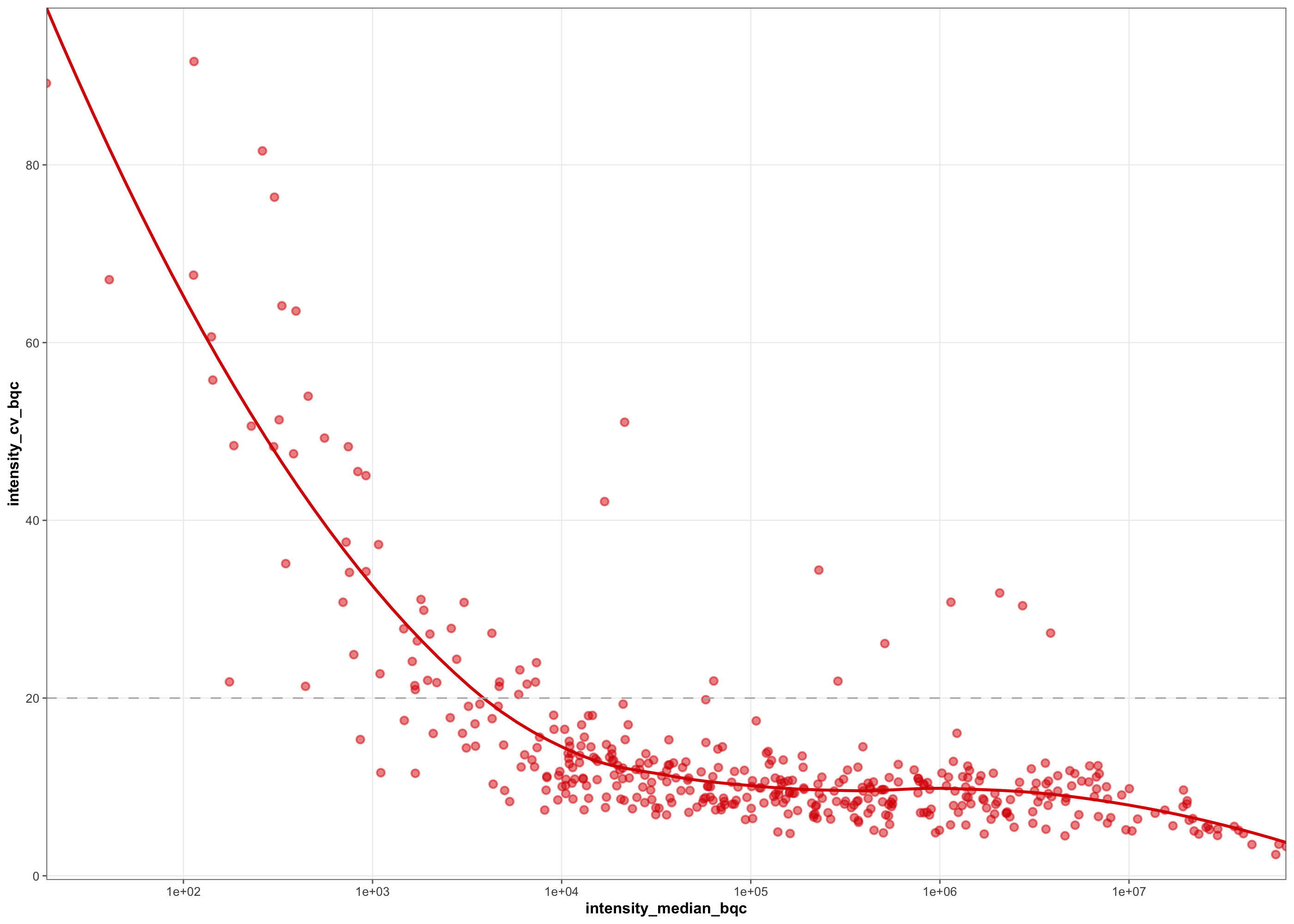
3.16 BQC vs TQC variability
Comparison of the variability in BQCs vs TQCs may be useful to understand the source of variability in the dataset (Broadhurst et al. 2018). If the variability in BQCs is much higher than in TQCs, this may suggest that the sample processing is a major contributor to overall variability. If the variability in TQCs and BQCs is similar, this may suggest that technical variability is a major contributor to overall variability. We look here at the sphingomyelins (SM), phosphatidylcholines (PC) and triglycerides (TG). PC and TG species consistently show higher variability in BQCs than in TQCs, suggesting that sample processing, i.e. lipid extraction, was a major contributor to overall variability, though it is unclear which factors in the sample processing contributed to it.
SMs, on the other hand, show similar variability in BQCs and TQCs, suggesting that sample processing contributed less to the overall variability for this class. This may be due to the fact that SMs are generally more abundant and thus less affected by variability in extraction efficiency.
mexp_temp <- calc_qc_metrics(
  mexp,
  use_robust_cv = TRUE, use_batch_medians = FALSE)
✔ QC metrics calculated for 477 features across 7 sample types, including normalized-intensity, concentration, and response-curve statistics.plot_qcmetrics_comparison(
mexp_temp,
plot_type = "diff",
y_shared = FALSE,
x_variable = "norm_intensity_cv_tqc",
y_variable = "norm_intensity_cv_bqc",
log_scale = FALSE, equality_line = TRUE,
facet_by_class = TRUE,
cols_page = 8, point_size = 1.3, font_base_size = 5, x_lim = c(0, 25),
y_lim = c(-6, 10),
legend_position = c(0.9, 0.10), legend_size = 0.7, strip_text_size = 8)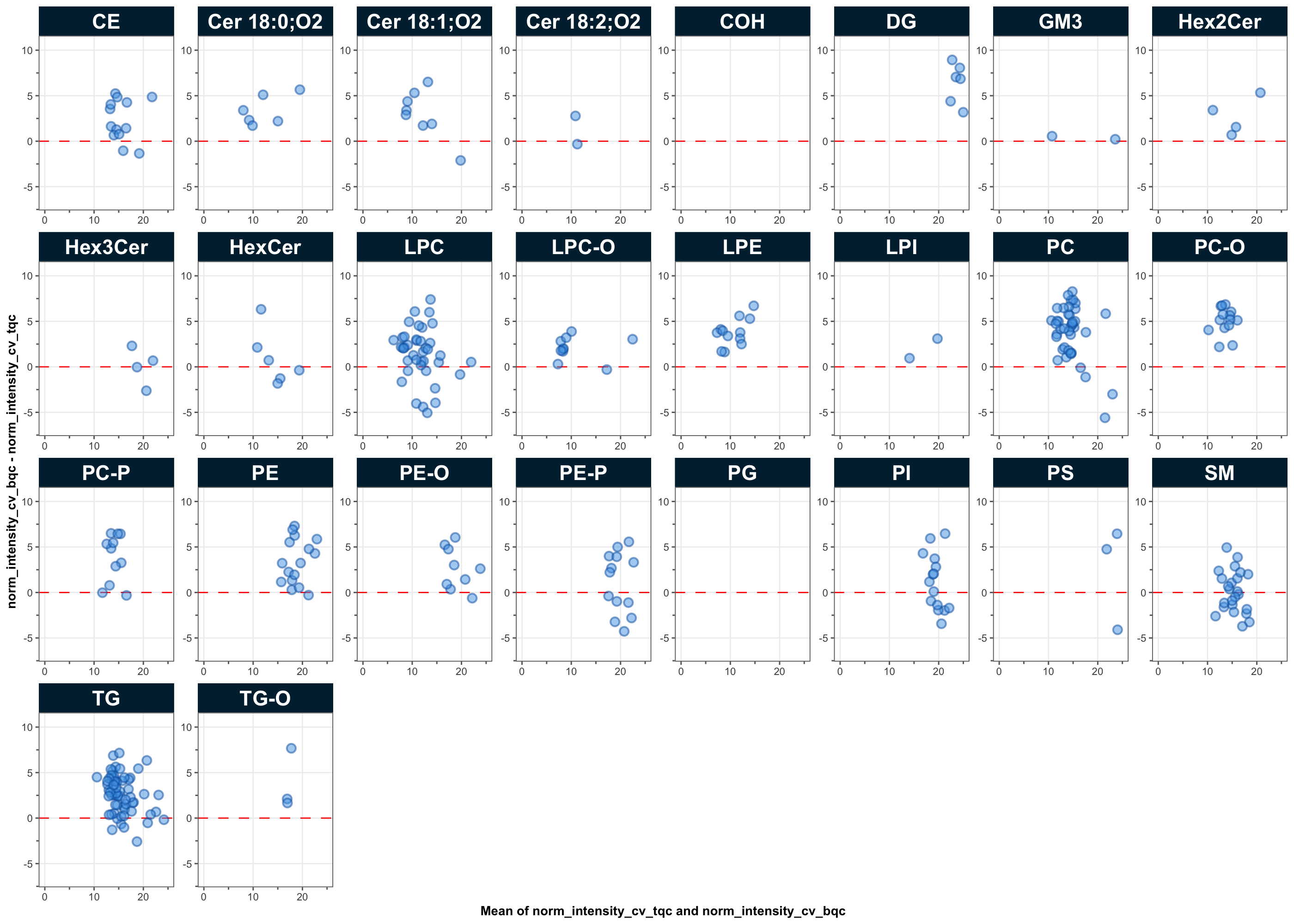
3.17 Response curves
Response curves relate the measured signal to the relative spiked-in amount and are used to assess the linear range and quantitative response of each analyte relative to its internal standard. The examples below show selected analytes together with their ISTDs.
sel_species <- c("PC 33:1 d7 (ISTD)", "PC 32:1", "PC 34:2", "PE 32:1")
mexp_temp <- mexp
mexp_temp@dataset <- mexp_temp@dataset %>%
  filter(feature_id %in% sel_species) %>%
  mutate(feature_id = factor(feature_id, levels = sel_species)) %>%
  arrange(feature_id)

mexp_temp@annot_responsecurves <- mexp_temp@annot_responsecurves |>
  filter(curve_id %in% c("A", "D"))

fig5f <- plot_responsecurves(
  data = mexp_temp,
  variable = "intensity",
  filter_data = FALSE,
  font_base_size = 4, line_width = 0.5, point_size = 1.2,
  include_feature_filter = sel_species,
  output_pdf = FALSE,
  show_progress = FALSE, cols_page = 2, rows_page = 2, return_plots = TRUE,
  legend_position = "inside-br", legend_size = 0.6, show_legend_title = FALSE,
  strip_text_size = 6)[[1]]
ℹ Generating plots (1 page)...✔ Donefig5f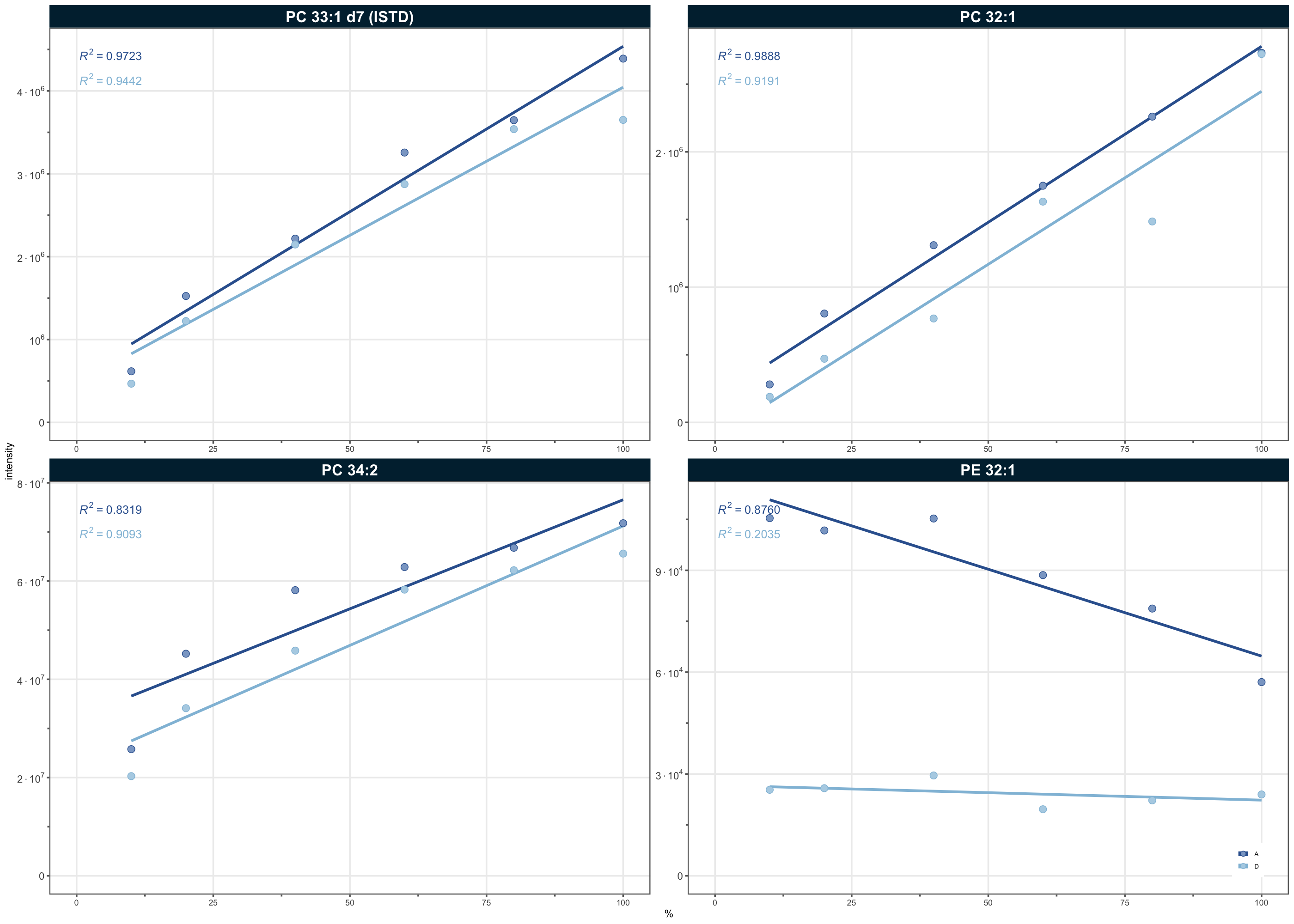
3.18 Feature filter
Features are now filtered on their QC metrics to retain only those meeting the quality criteria for the final dataset. The thresholds below combine several criteria: an adequate response-curve fit (R² ≥ 0.8, slope ≥ 0.5, y-intercept ≤ 0.5), sufficient signal over blank (≥ 10) and absolute intensity (≥ 100), and acceptable precision in the batch QCs (CV ≤ 25 %). A few cholesteryl esters that fail these criteria are retained explicitly via features.to.keep, as they are of specific interest for this study; their higher variability is noted below.
mexp_final <- filter_features_qc(
  data = mexp,
  recalc_metrics = TRUE, clear_existing = TRUE, use_batch_medians = TRUE,
  include_qualifier = FALSE,
  include_istd = FALSE,
  response.curves.selection = c(1, 2),
  response.curves.summary = "mean",
  min.rsquare.response = 0.8,
  min.slope.response = 0.5,
  max.yintercept.response = 0.5,
  min.signalblank.median.spl.pblk = 10,
  min.intensity.median.spl = 100,
  max.cv.conc.bqc = 25,
  max.dratio.sd.conc.bqc = 0.75,
  max.prop.missing.conc.spl = 100,
  features.to.keep = c(
    "CE 20:4",
    "CE 22:5", "CE 22:6", "CE 16:0", "CE 18:0"))
! %CV not computed for 11270 feature×QC-type×variable combinations with fewer than 3 replicates (LTR: 11267, TQC: 3).✔ QC metrics calculated for 477 features across 7 sample types, including normalized-intensity, concentration, and response-curve statistics.! The QC parameter min.intensity.median.spl contains NAs for the following features: COH d7 [161] (ISTD), DG 14:1_20:0 [-20:0], DG 18:1_20:0 [-18:1], Hex2Cer d18:.... These features failed QC.! The QC parameter min.signalblank.median.spl.pblk contains NAs for the following features: COH d7 [161] (ISTD), DG 14:1_20:0 [-20:0], DG 18:1_20:0 [-18:1], Hex2Cer d18:.... These features failed QC.! The QC parameter max.cv.conc.bqc contains NAs for the following features: Cer d18:1/12:0 (ISTD) [M-H20>264], Cer d18:1/25:0 (ISTD) [M-H20>264], COH [16.... These features failed QC.! The QC parameter max.dratio.sd.conc.bqc contains NAs for the following features: CE 18:1 d7 (ISTD), Cer d18:1/12:0 (ISTD) [M-H20>264], Cer d18:1/25:0 (ISTD), .... These features failed QC.! The QC parameter max.prop.missing.conc.spl contains NAs for the following features: DG 14:1_20:0 [-20:0], DG 18:1_20:0 [-18:1], Hex2Cer d18:1/16:0 d3 (ISTD) [-He.... These features failed QC.! The following features were forced to be retained despite not meeting filtering criteria: CE 16:0, CE 18:0, CE 20:4, CE 22:5, and CE 22:6✔
New feature QC filters were defined: 314 of 412 quantifier features meet QC criteria (not including the 18 quantifier ISTD features).3.19 Feature filter Results
How many analytes passed and failed the QC criteria, per lipid class.
lipidCat_order <- c(
  "Cer 18:0;O2",
  "Cer 18:1;O2", "Cer 18:2;O2", "SM", "Hex2Cer", "Hex3Cer", "HexCer", "GM3",
  "LPC", "LPE", "LPI", "LPC-O", "PC", "PE", "PI", "PG", "PS", "PC-O",
  "PC-P", "PE-O", "PE-P", "DG", "TG", "TG-O", "COH", "CE")

mexp_final@metrics_qc$feature_class <- factor(
  mexp_final@metrics_qc$feature_class,
  lipidCat_order)
mexp_final@metrics_qc <- mexp_final@metrics_qc |> arrange(feature_class)

fig5h <- plot_qc_summary_byclass(
  mexp_final,
  font_base_size = 6, legend_position = c(0.77, 0.27), legend_size = 0.7,
  show_legend_title = FALSE)
fig5h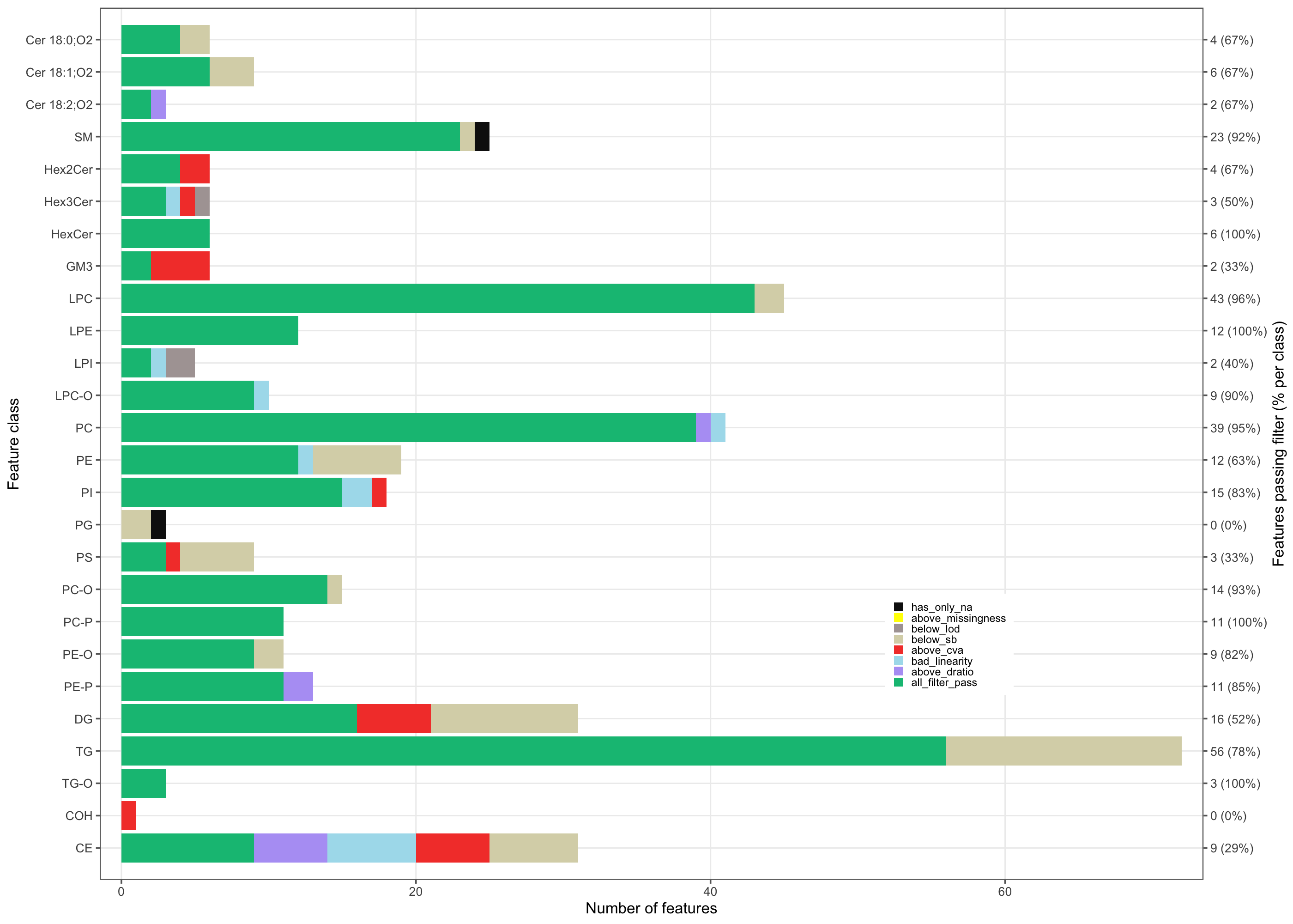
3.20 Overview analytical variability
The analytical variability of the filtered dataset, as the distribution of coefficients of variation (CVs) in the BQCs for all features. The cholesteryl esters (CE), which were retained in the final dataset despite failing QC, show higher variability. This must be taken into account in subsequent statistical analyses and interpretation.
plot_abundanceprofile(
  data = mexp_final,
  use_qc_metrics = TRUE, log_scale = FALSE,
  filter_data = TRUE,
  variable = "conc_cv_bqc",
  density_strip = TRUE,
  qc_types = "SPL",
  #analysis_range = c(1,4000),
  show_sum = FALSE,
  #x_lim = c(6.5, 7.5),
  x_label = NA,
  feature_map = "lipidomics")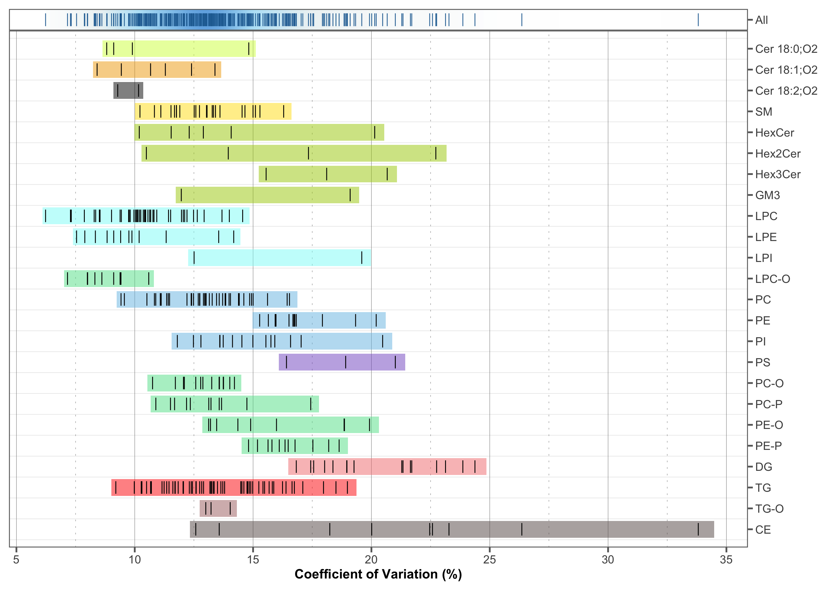
3.21 Feature filter Venn
How many features passed or failed across all criteria, and how the individual QC criteria overlapped in the features they removed.
fig5ex <- plot_qc_summary_overall(mexp_final)

fig5g <- fig5ex[[2]] +
  theme(
    strip.text = ggplot2::element_text(size = 5),
    #aspect.ratio = 0.9,
    legend.position = "inside", axis.text = element_text(size = 4),
    axis.title = element_text(size = 6), legend.direction = "vertical",
    legend.text = element_text(size = 6 * 0.7),
    legend.title = element_text(size = 6 * 0.7),
    legend.key.size = unit(6 * 0.7, "pt"))

fig5g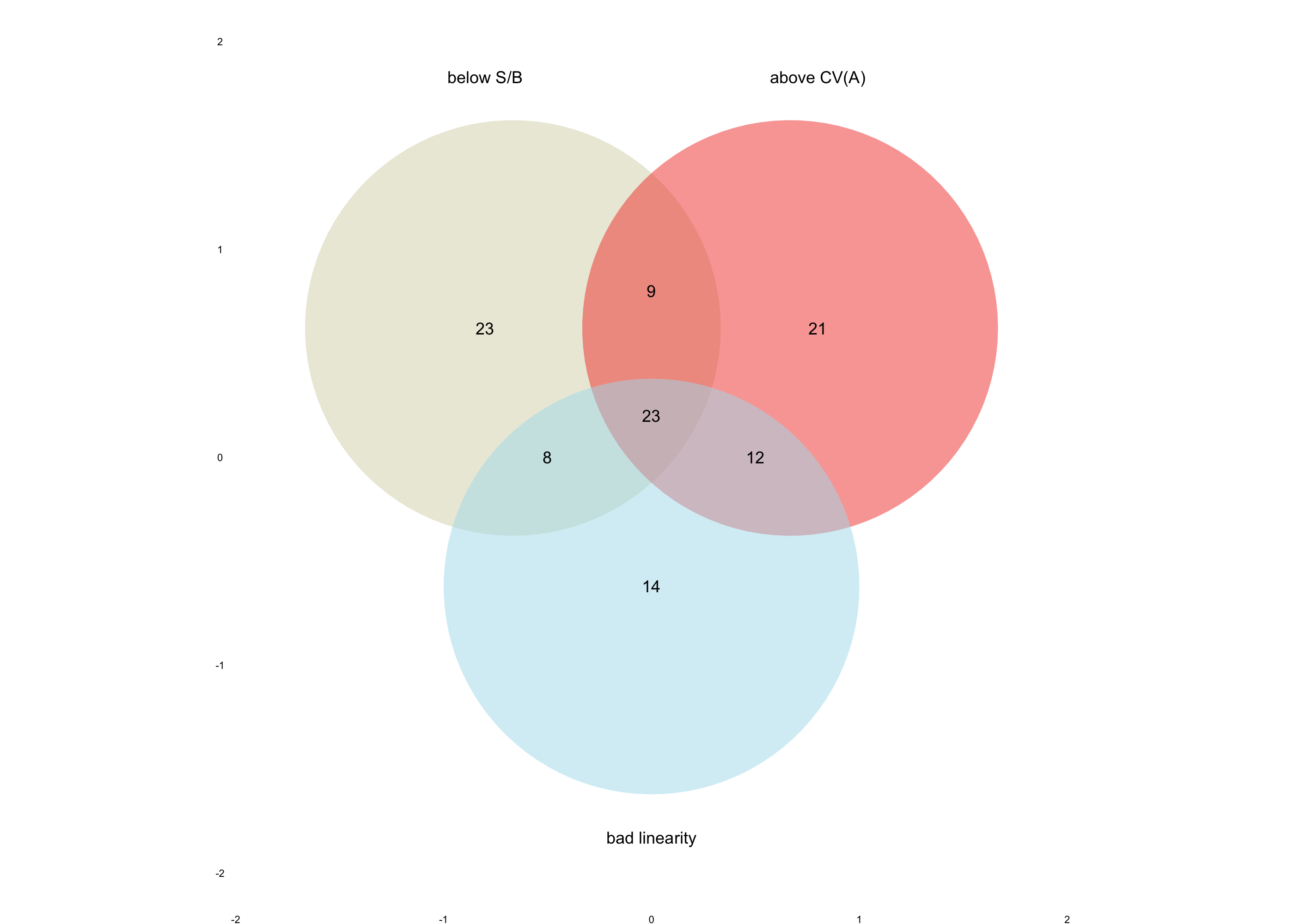
3.22 Lipidome Profile
As a final overview, the feature concentration profile of the filtered dataset is shown below. Validating the concentrations, for example, those of the most abundant species, the summed concentrations per lipid class, or the ratios between lipid classes, against in-house reference values or literature data helps ensure that the quantification is within expected ranges and that no major quantification errors are present.
fig5i <- plot_abundanceprofile(
  data = mexp_final,
  log_scale = TRUE,
  variable = "conc",
  filter_data = TRUE,
  qc_types = "SPL",
  #x_lim = c(-6, 2),
  x_label = NA, font_base_size = 6,
  feature_map = "lipidomics")

fig5i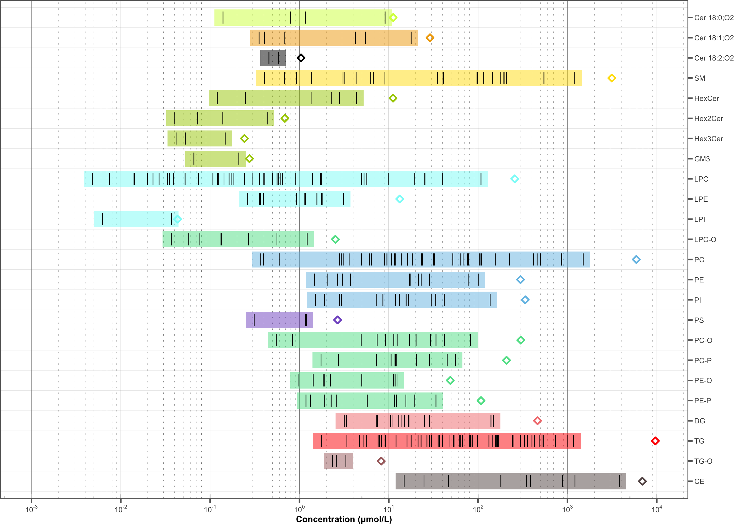
3.23 Exporting the dataset
The dataset is exported as a CSV file. The user can specify the variable to export, whether to include qualifier features, whether to restrict the output to specific QC types (here the study samples, SPL), and whether to apply the QC feature filter.
Two versions are written here. The first contains the uncorrected concentrations (conc_raw) of all features, before the QC filter, which is useful for re-examining features that did not pass QC.
save_dataset_csv(
  data = mexp,
  path = "./output/Dataset1_UNFILTERED_RAW-feature_conc_uM.csv",
  variable = "conc_raw",
  qc_types = "SPL",
  include_qualifier = FALSE,
  filter_data = FALSE)
✔ Conc_raw values for 678 analyses and 412 features have been exported to './output/Dataset1_UNFILTERED_RAW-feature_conc_uM.csv'.The second is the final dataset: drift- and batch-corrected concentrations (conc) restricted to the features that passed the QC filter (filter_data = TRUE), taken from the filtered object mexp_final.
save_dataset_csv(
  data = mexp_final,
  path = "./output/Dataset1_FILTERED-feature_conc_uM.csv",
  variable = "conc",
  qc_types = "SPL",
  include_qualifier = FALSE,
  filter_data = TRUE)
✔ Concentration values for 678 analyses and 314 features have been exported to './output/Dataset1_FILTERED-feature_conc_uM.csv'.The complete MRMhubExperiment — imported data, metadata and all processing results — is also saved as a single .rds with save_dataset_rds(). This self-contained object can be shared and reopened in any R session with read_dataset_rds(), which verifies an embedded integrity hash, to continue or audit the analysis without re-running the pipeline.
save_dataset_rds(mexp, "./output/Dataset1_mexp.rds")✔ MRMhubExperiment saved to ./output/Dataset1_mexp.rds.Content fingerprint: "c8dd3e9b18bbb76bdcbb4c50fc8a80d7"4 Figures for the manuscript in preparation
Note: the code and corresponding plots below are used for a manuscript currently in preparation.
4.1 Assembling Figure 4
fig4 <- ((fig4a | fig4b) /
  ((fig4c | fig4d | fig4e) + plot_layout(widths = c(0.9, 0.9, 1))) /
  ((fig4f | fig4g) + plot_layout(widths = c(1.07, 0.93)))) +
  plot_layout(heights = c(1, 0.9, 1)) +
  plot_annotation(tag_levels = 'a') +
  theme(
    plot.tag = element_text(size = 12, face = "bold"),
    strip.placement = 'inside')

save_plot(
  fig4, "output/fig4", format = c("pdf", "png"),
  width = 180, height = 200, show_plot = FALSE)
✔ Saved plot (180 x 200 mm) to output/fig4.pdf, output/fig4.png4.2 Assembling Figure 5
layout <- "
AABB
CCDD
EEFF
"

fig5 <- (fig5a | fig5b) /
  #(p_fig2c | p_fig2d) /
  (fig5c | fig5d) /
  ((fig5e |
    fig5f |
    (fig5g +
      theme(axis.text = element_blank(), axis.title = element_blank()))) +
    plot_layout(widths = c(1.0, 1.1, 0.9))) /
  (fig5h | fig5i) +
  plot_layout(heights = c(0.8, 1, 0.9, 1.5)) +
  plot_annotation(tag_levels = 'a') +
  theme(
    plot.tag = element_text(size = 10, face = "bold"),
    strip.placement = 'inside')
save_plot(
  fig5, "output/fig5", format = c("pdf", "png"),
  width = 180, height = 240)
`geom_smooth()` using formula = 'y ~ x'
`geom_smooth()` using formula = 'y ~ x'
✔ Saved plot (180 x 240 mm) to output/fig5.pdf, output/fig5.png
`geom_smooth()` using formula = 'y ~ x'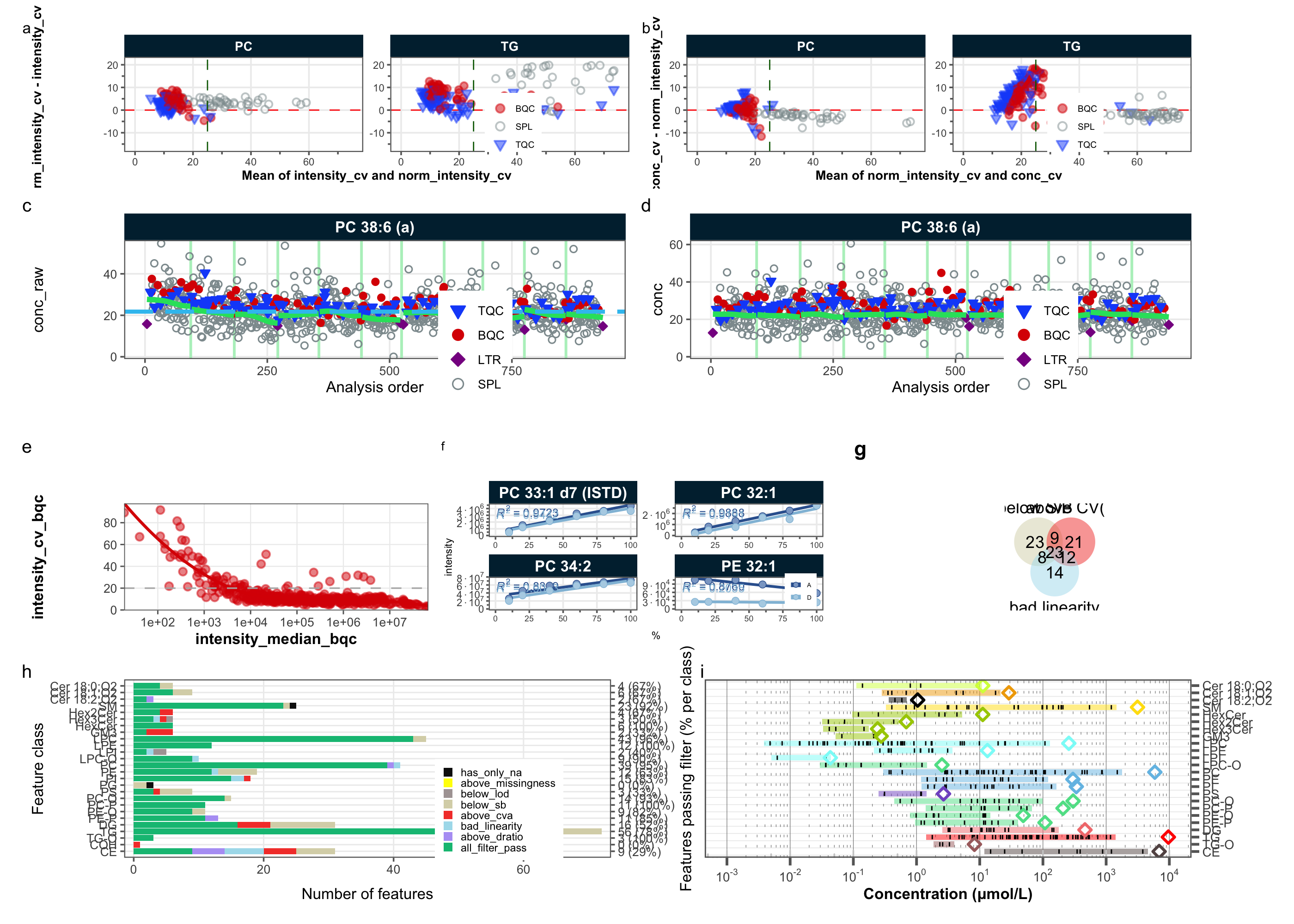
output/fig5.{png,pdf} (180 mm).
4.3 Assembling Extended Figure 4
# include fig4b again as extfig4a for better comparison of RLAs before and after normalization
extfig4a <- fig4b

extfig4 <- (extfig4a / extfig4b / extfig4c / extfig4d) +
  plot_layout(ncol = 1, heights = c(1, 1, 1, 1)) +
  plot_annotation(tag_levels = 'a') +
  theme(
    plot.tag = element_text(size = 19, face = "bold"),
    strip.placement = 'inside')

save_plot(
  extfig4, "output/ExtendedFig-4_RLAs.pdf",
  width = 180, height = 250)
✔ Saved plot (180 x 250 mm) to output/ExtendedFig-4_RLAs.pdf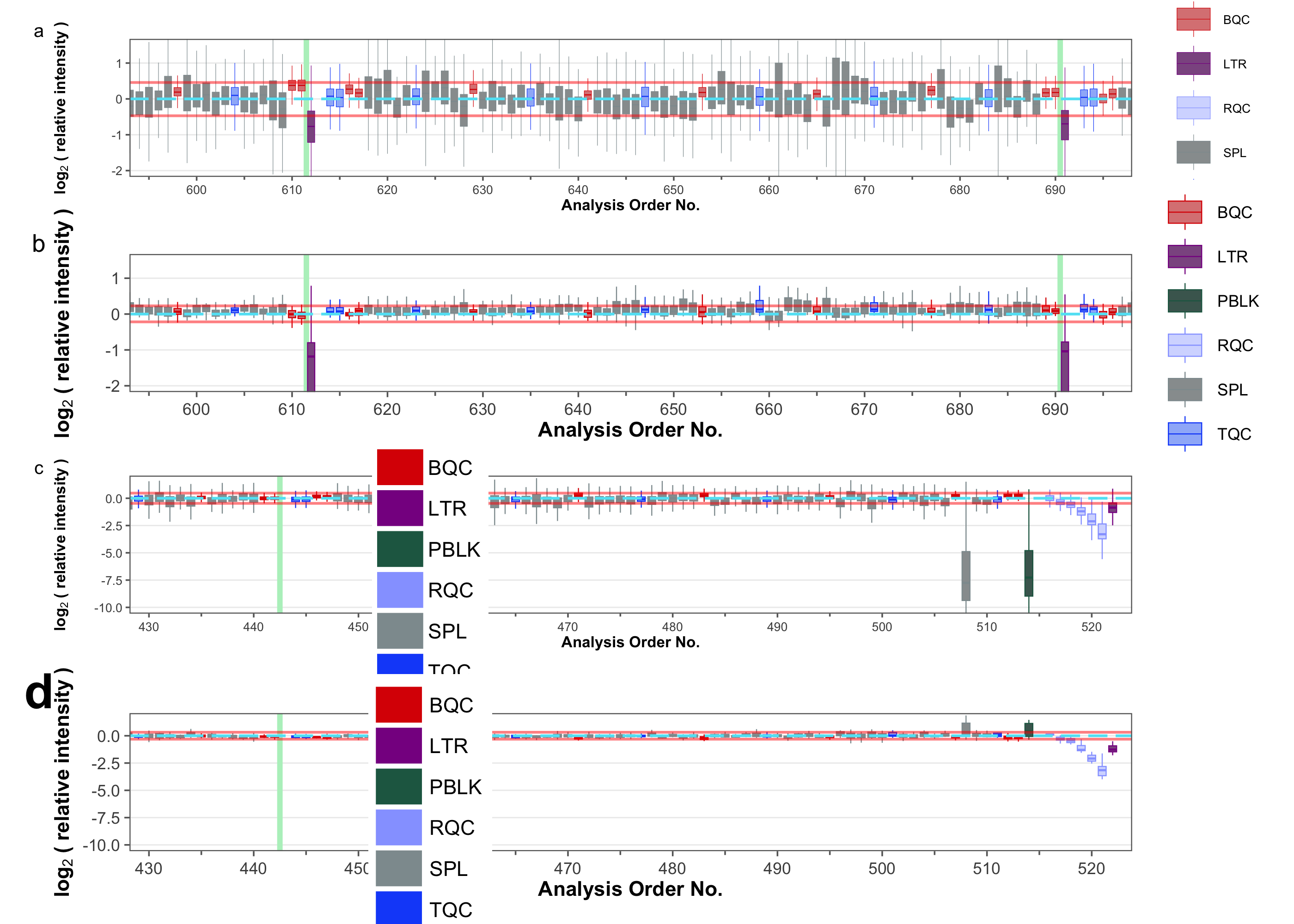
output/ExtendedFig-4_RLAs.pdf.
4.4 Assembling Extended Figure 5
extfig5 <- extfig5a /
  extfig5b +
  plot_annotation(tag_levels = 'a') +
  theme(
    plot.tag = element_text(size = 12, face = "bold"),
    strip.placement = 'inside')

save_plot(
  extfig5, "output/ExtendedFig-5.png",
  width = 180, height = 250)
✔ Saved plot (180 x 250 mm) to output/ExtendedFig-5.png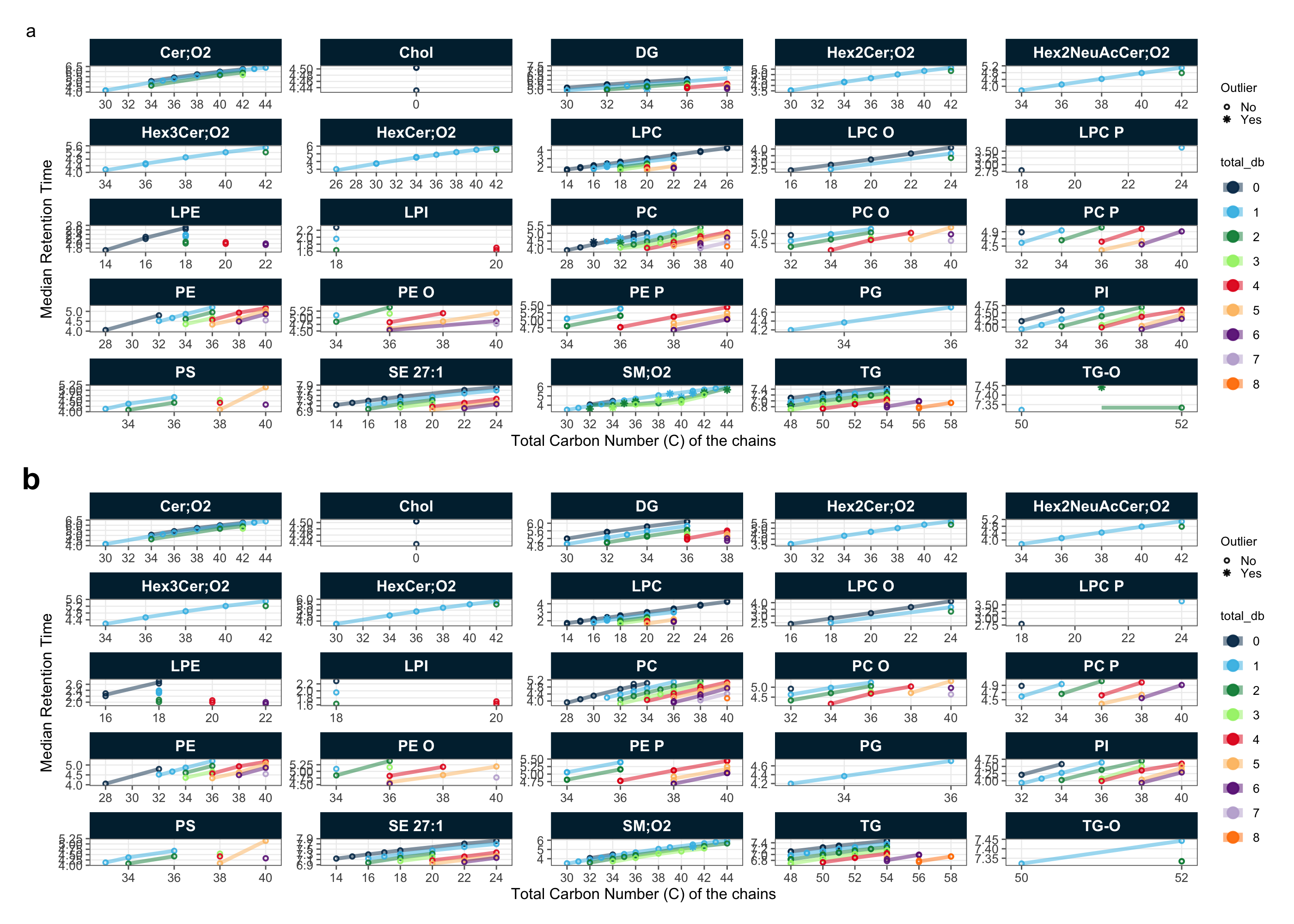
output/ExtendedFig-5.png.
4.5 Assembling Extended Figure 6
extfig6 <- extfig6a /
  extfig6b +
  plot_layout(ncol = 1, heights = c(1, 1.5)) +
  plot_annotation(tag_levels = 'a') +
  theme(
    plot.tag = element_text(size = 12, face = "bold"),
    strip.placement = 'inside')

save_plot(
  extfig6, "output/ExtendedFig-6_PCAloading", format = c("pdf", "png"),
  width = 180, height = 250)
✔ Saved plot (180 x 250 mm) to output/ExtendedFig-6_PCAloading.pdf, output/ExtendedFig-6_PCAloading.png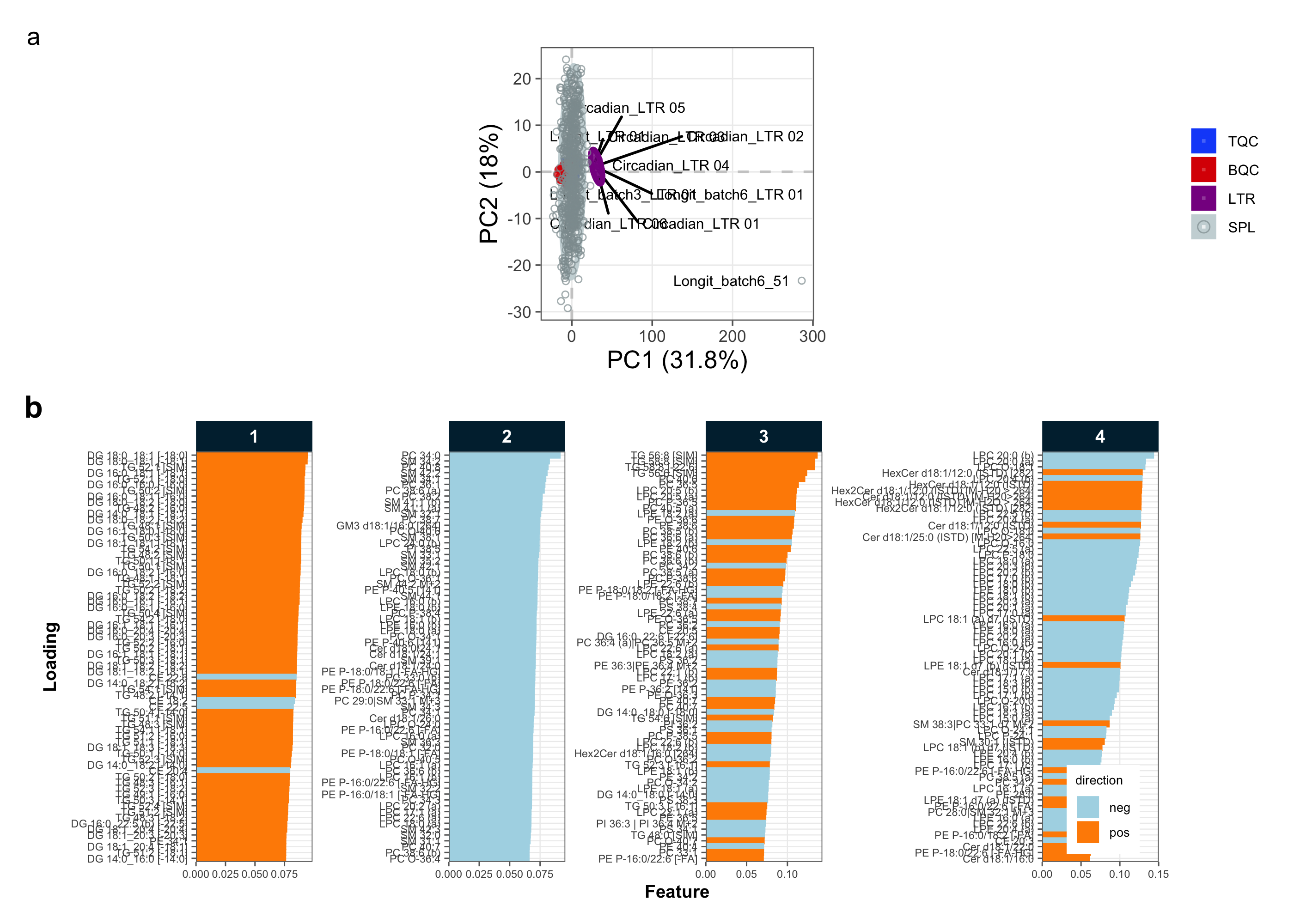
output/ExtendedFig-6_PCAloading.{png,pdf}.
4.6 Saving Extended Figure 7
save_plot(
  extfig7[[1]], "output/ExtendedData_Fig7_ISTDtrends.png",
  width = 180, height = 180, show_plot = FALSE)
✔ Saved plot (180 x 180 mm) to output/ExtendedData_Fig7_ISTDtrends.png4.7 Assembling Extended Figure 8
extfig8 <- extfig8a /
  extfig8b /
  extfig8c +
  plot_layout(ncol = 1, heights = c(1, 1, 1)) +
  plot_annotation(tag_levels = 'a') +
  theme(
    plot.tag = element_text(size = 12, face = "bold"),
    strip.placement = 'inside')
save_plot(
  extfig8, "output/ExtendedData_Fig8_CVnormbeforeafter.pdf",
  width = 160, height = 270)
✔ Saved plot (160 x 270 mm) to output/ExtendedData_Fig8_CVnormbeforeafter.pdf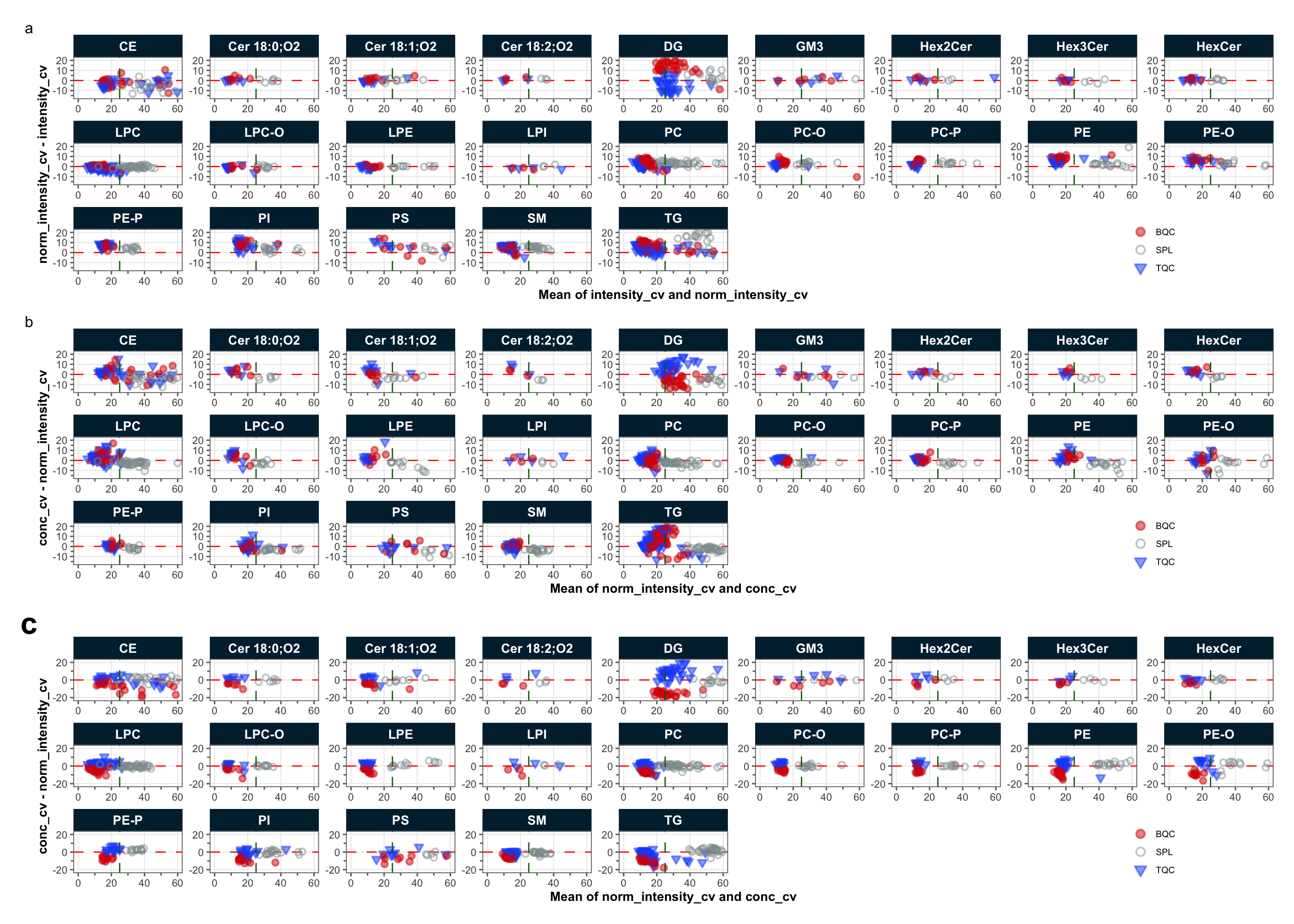
output/ExtendedData_Fig8_CVnormbeforeafter.pdf.
5 Supplementary Figures of Manuscript
5.1 Runscatter plots
plot_runscatter(
  mexp,
  variable = "intensity",
  qc_types = c("SPL", "BQC", "TQC", "LTR"),
  show_reference_lines = TRUE,
  ref_qc_types = "SPL",
  reference_fill_color = "#111111", reference_k_sd = 3, show_trend = FALSE,
  point_size = 1.2, font_base_size = 6, cols_page = 3, rows_page = 3,
  cap_outliers = TRUE, reference_sd_shade = FALSE,
  #batch_zebra_stripe = TRUE,
  show_progress = FALSE,
  multithreading = FALSE, # set TRUE (needs mirai, carrier, qpdf) to parallelise PDF export across mirai daemons
  output_pdf = TRUE,
  path = "output/suppl-fig1_runscatter_area.pdf",
  return_plots = FALSE)

plot_runscatter(
  mexp,
  variable = "conc_raw",
  qc_types = c("SPL", "BQC", "TQC", "LTR"),
  show_reference_lines = TRUE,
  ref_qc_types = "SPL",
  reference_fill_color = "#111111", reference_k_sd = 3, show_trend = TRUE,
  point_size = 1.2, font_base_size = 6, cols_page = 3, rows_page = 3,
  cap_outliers = TRUE, reference_sd_shade = FALSE,
  #batch_zebra_stripe = TRUE,
  show_progress = FALSE,
  multithreading = FALSE, # set TRUE (needs mirai, carrier, qpdf) to parallelise PDF export across mirai daemons
  output_pdf = TRUE,
  path = "output/suppl-fig2_runscatter_conc-raw.pdf",
  return_plots = FALSE)

plot_runscatter(
  mexp,
  variable = "conc",
  qc_types = c("SPL", "BQC", "TQC", "LTR"),
  show_reference_lines = TRUE,
  ref_qc_types = "SPL",
  reference_fill_color = "#111111", reference_k_sd = 3, show_trend = TRUE,
  point_size = 1.2, font_base_size = 6, cols_page = 3, rows_page = 3,
  cap_outliers = TRUE, reference_sd_shade = FALSE,
  #batch_zebra_stripe = TRUE,
  show_progress = FALSE,
  multithreading = FALSE, # set TRUE (needs mirai, carrier, qpdf) to parallelise PDF export across mirai daemons
  output_pdf = TRUE,
  path = "output/suppl-fig3_runscatter_conc-final.pdf",
  return_plots = FALSE)
6 References
Broadhurst, David, Royston Goodacre, Stacey N. Reinke, et al. 2018. “Guidelines and Considerations for the Use of System Suitability and Quality Control Samples in Mass Spectrometry Assays Applied in Untargeted Clinical Metabolomic Studies.” Metabolomics 14 (6): 72. https://doi.org/10.1007/s11306-018-1367-3.
De Livera, Alysha M., Daniel A. Dias, David De Souza, et al. 2012. “Normalizing and Integrating Metabolomics Data.” Analytical Chemistry 84 (24): 10768–76. https://doi.org/10.1021/ac302748b.
Livera, Alysha M. De, Marko Sysi-Aho, Laurent Jacob, et al. 2015. “Statistical Methods for Handling Unwanted Variation in Metabolomics Data.” Analytical Chemistry 87 (7): 3606–15. https://doi.org/10.1021/ac502439y.
Tan, Sock Hwee, Hiromi W. L. Koh, Jing Yi Chua, et al. 2022. “Variability of the Plasma Lipidome and Subclinical Coronary Atherosclerosis.” Arteriosclerosis, Thrombosis, and Vascular Biology 42 (1): 100–112. https://doi.org/10.1161/ATVBAHA.121.316847.