Quantitative assay with Ext. calibration and QC • midar

This vignette demonstrates a simple workflow for a quantitative targeted assay with external calibration and quality control samples, as used in e.g. in clinical chemistry or environmental analysis.

For this type of analysis the known/target concentrations for the calibrator and QC samples must be defined in the QCconcentrations metadata. This also required that sample_id and analyte_id is defined for the corresponding analyses in the analysis, and for the features in the feature metadata tables, respectively.

Quality control concentration plot

So, we first import the data and metadata from a MassHunter CSV file and an MsOrganiser template file. The datasets used in this example can be obtained from https://github.com/SLINGhub/midar/tree/main/data-raw.

library(midar)

# Create a new MidarExperiment data object
mexp <- MidarExperiment(title = "Corticosteroid Assay")

# Import analysis data (peak integration results) from a MassHunter CSV file
mexp <- import_data_masshunter(
  data = mexp,
  path = "QuantLCMS_Example_MassHunter.csv",
  import_metadata = TRUE)
#> indexed 0B in  0s, 0B/sindexed 1.00TB in  0s, 3.46PB/s                                                                              

# Import metadata from an msorganiser template fie
mexp <- import_metadata_msorganiser(
  mexp,
  path = "QuantLCMS_Example_Metadata.xlsm",
  excl_unmatched_analyses = T, ignore_warnings = T)
#> --------------------------------------------------------------------------------------------
#>   Type Table    Column    Issue                        Count
#> 1 N    Analyses sample_id Not defined for all analyses     8
#> --------------------------------------------------------------------------------------------
#> E = Error, W = Warning, W* = Supressed Warning, N = Note
#> --------------------------------------------------------------------------------------------

Next, the raw peak areas are normalized with the corresponding internal standard and then we calculate and plot the regression fits for the external calibration curves.

# Normalize data by internal standards (defined in feature metadata)
mexp <- normalize_by_istd(mexp)

# Calculate calibration results. The regression model and weighting 
# can also be specified per feature in the feature metadata
mexp <- calc_calibration_results(
  mexp, 
  fit_overwrite  = TRUE,  # Set to FALSE if defined in metadata
  fit_model = "quadratic", 
  fit_weighting = "1/x")

# Plot calibration curves
  p <- plot_calibrationcurves(
    data = mexp,
    fit_model = "quadratic",
    fit_weighting = "1/x",
    rows_page = 2,
    cols_page = 4, show_progress = FALSE
  )

Calibration plots

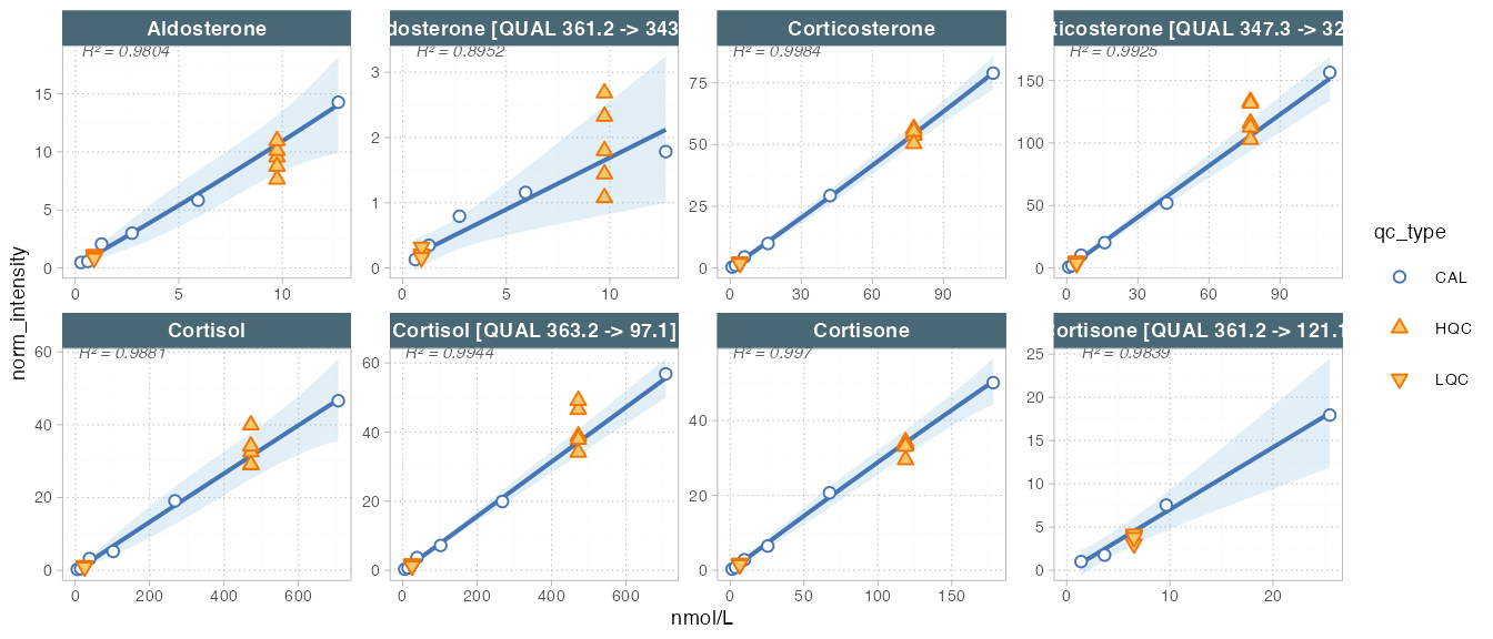
We also can output a summary of the calibration curve results:

tbl_cal <- get_calibration_metrics(mexp)
tbl_cal
#> # A tibble: 8 × 14
#>   feature_id   is_quantifier fit_model fit_weighting reg_failed    r2 lowest_cal
#>   <chr>        <lgl>         <chr>     <chr>         <lgl>      <dbl>      <dbl>
#> 1 Aldosterone  TRUE          quadratic 1/x           FALSE      0.980      0.277
#> 2 Aldosterone… FALSE         quadratic 1/x           FALSE      0.981      0.277
#> 3 Corticoster… TRUE          quadratic 1/x           FALSE      0.998      0.867
#> 4 Corticoster… FALSE         quadratic 1/x           FALSE      0.994      0.867
#> 5 Cortisol     TRUE          quadratic 1/x           FALSE      0.988      5.52 
#> 6 Cortisol [Q… FALSE         quadratic 1/x           FALSE      0.995      5.52 
#> 7 Cortisone    TRUE          quadratic 1/x           FALSE      0.997      1.39 
#> 8 Cortisone [… FALSE         quadratic 1/x           FALSE      0.984      1.39 
#> # ℹ 7 more variables: highest_cal <dbl>, coef_a <dbl>, coef_b <dbl>,
#> #   coef_c <dbl>, lod <dbl>, loq <dbl>, sigma <dbl>

After we have inspected the curves and are happy with the quality of the analysis, we can calculate the concentrations for all features in samples using the external calibration curves.

A summary of the QC results (bias and variability) is calculated and shown below. The final concentration data is saved to a CSV file.

# Calculate concentrations for all samples using external calibration
mexp <- quantify_by_calibration(
  mexp,
  fit_overwrite = FALSE,
  include_qualifier = FALSE,
  ignore_failed_calibration = TRUE,
  fit_model = "quadratic",
  fit_weighting = "1/x")

# get a table with QC results (bias and variability)
tbl <- get_qc_bias_variability(mexp, qc_types = c("HQC", "LQC"))

# Save a table with final concentration data
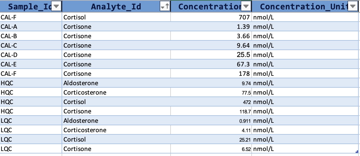
 save_dataset_csv( mexp, 
                   path = "corticosteroid_conc.csv", 
                   variable = "conc", 
                   filter_data = FALSE)
 
 print(tbl)
#> # A tibble: 8 × 9
#>   feature_id     sample_id qc_type     n conc_target conc_mean conc_sd cv_intra
#>   <chr>          <chr>     <chr>   <int>       <dbl>     <dbl>   <dbl>    <dbl>
#> 1 Aldosterone    HQC       HQC         5       9.74      8.65    1.14     13.1 
#> 2 Aldosterone    LQC       LQC         5       0.911     0.843   0.132    15.7 
#> 3 Corticosterone HQC       HQC         5      77.5      77.3     3.15      4.08
#> 4 Corticosterone LQC       LQC         5       4.11      3.53    0.376    10.7 
#> 5 Cortisol       HQC       HQC         5     472       495.     68.3      13.8 
#> 6 Cortisol       LQC       LQC         5      25.2      20.0     2.40     12.0 
#> 7 Cortisone      HQC       HQC         5     119.      114.      6.73      5.89
#> 8 Cortisone      LQC       LQC         5       6.52      6.23    0.504     8.08
#> # ℹ 1 more variable: bias <dbl>