MiDAR is an R package designed for the reproducible
post-processing, quality control, and reporting of quantitative
small-molecule mass spectrometry (MS) data. Its modular functionalities
and defined data structure, support diverse analytical designs, data
formats, and processing tasks, including metabolomics and lipidomics.
MiDAR is intended for both analytical and bioinformatics
scientists and to facilitate collaboration between them. It enables the
creation of customizable, supervisable, and documented data processing
workflows through intuitive high-level R functions and data objects.
MiDAR’s core tools, accessible also to those with
limited R experience, allow analysts to annotate, inspect, and process
data. This includes importing data and metadata from various file
formats, managing and organizing data with integrity checks, performing
processing tasks such as quantification, drift/batch correction, and
applying QC-based feature filtering. Users can assess data quality using
QC metrics and diagnostic plots, and share both raw and processed data
along with the entire processing workflow for further analyses and
documentation.
MiDAR also serves as a software library for building
robust and scalable data processing pipelines.
Getting Started
Visit the MiDAR Documentation page (https://slinghub.github.io/midar) for a detailed introduction and comprehensive documentation on this package.
Installation
if (!require("pak")) install.packages("pak")
pak::pkg_install("SLINGhub/midar")
Example Workflow
# Path of example files included with this package
dir_path <- system.file("extdata", package = "midar")
# Create a MidarExperiment object
mexp <- MidarExperiment()
# Load data and metadata
mexp <- import_data_mrmkit(mexp,
path = file.path(dir_path, "MRMkit_demo.tsv"),
import_metadata = TRUE)
#> ✔ Imported 499 analyses with 28 features
#> ℹ `feature_area` selected as default feature intensity. Modify with `set_intensity_var()`.
#> ✔ Analysis metadata associated with 499 analyses.
#> ✔ Feature metadata associated with 28 features.
mexp <- import_metadata_analyses(mexp,
path = file.path(dir_path, "MRMkit_AnalysesAnnot.csv"),
ignore_warnings = T)
#> ✔ Analysis metadata associated with 499 analyses.
#> ✔ Feature metadata associated with 28 features.
mexp <- import_metadata_istds(mexp,
path = file.path(dir_path, "MRMkit_ISTDconc.csv"))
#> ✔ Analysis metadata associated with 499 analyses.
#> ✔ Feature metadata associated with 28 features.
#> ✔ Internal Standard metadata associated with 9 ISTDs.
# Normalize and quantitate features by internal standards
mexp <- normalize_by_istd(mexp)
#> ✔ 19 features normalized with 9 ISTDs in 499 analyses.
mexp <- quantify_by_istd(mexp)
#> ✔ 19 feature concentrations calculated based on 9 ISTDs and sample amounts of 499 analyses.
#> ℹ Concentrations are given in μmol/L.
# Drift and batch-effect correction
mexp <- correct_drift_cubicspline(mexp, variable = "conc", ref_qc_types = "BQC")
#> ℹ Applying `conc` drift correction...
#> | | | 0% | |= | 3% | |== | 5% | |=== | 8% | |===== | 11% | |====== | 13% | |======= | 16% | |======== | 18% | |========= | 21% | |========== | 24% | |============ | 26% | |============= | 29% | |============== | 32% | |=============== | 34% | |================ | 37% | |================= | 39% | |=================== | 42% | |==================== | 45% | |===================== | 47% | |====================== | 50% | |======================= | 53% | |======================== | 55% | |========================= | 58% | |=========================== | 61% | |============================ | 63% | |============================= | 66% | |============================== | 68% | |=============================== | 71% | |================================ | 74% | |================================== | 76% | |=================================== | 79% | |==================================== | 82% | |===================================== | 84% | |====================================== | 87% | |======================================= | 89% | |========================================= | 92% | |========================================== | 95% | |=========================================== | 97% | |============================================| 100% - trend smoothing done!
#> ✔ Drift correction was applied to 19 of 19 features (batch-wise).
#> ℹ The median CV change of all features in study samples was 0.57% (range: -0.72% to 2.66%). The median absolute CV of all features across batches increased from 33.20% to 35.31%.
mexp <- correct_batch_centering(mexp, variable = "conc", ref_qc_types = "BQC")
#> ℹ Adding batch correction on top of `conc` drift-correction.
#> ✔ Batch median-centering of 6 batches was applied to drift-corrected concentrations of all 19 features.
#> ℹ The median CV change of all features in study samples was 0.01% (range: -7.60% to 2.50%). The median absolute CV of all features increased from 36.14% to 36.76%.
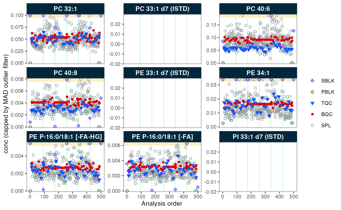
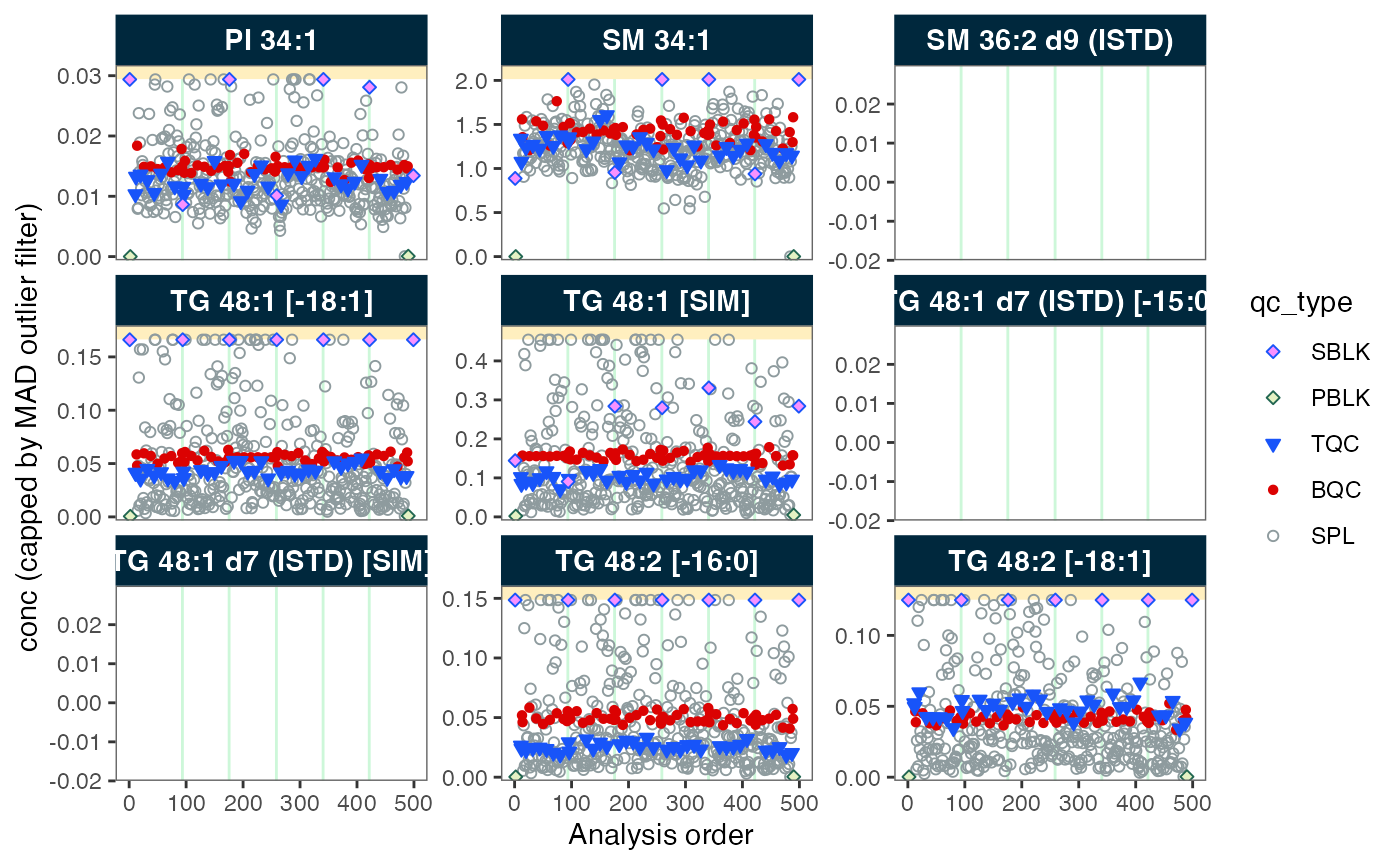
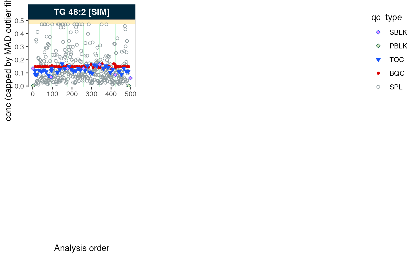
# Plot analysis time-trends of final concentrations of each feature
plot_runscatter(mexp,
variable = "conc",
qc_types = c("BQC", "TQC", "SPL", "PBLK", "SBLK"),
cap_outliers = TRUE,
output_pdf = FALSE,
path = "./output/runscatter_istd.pdf")
#> Generating plots (4 pages)...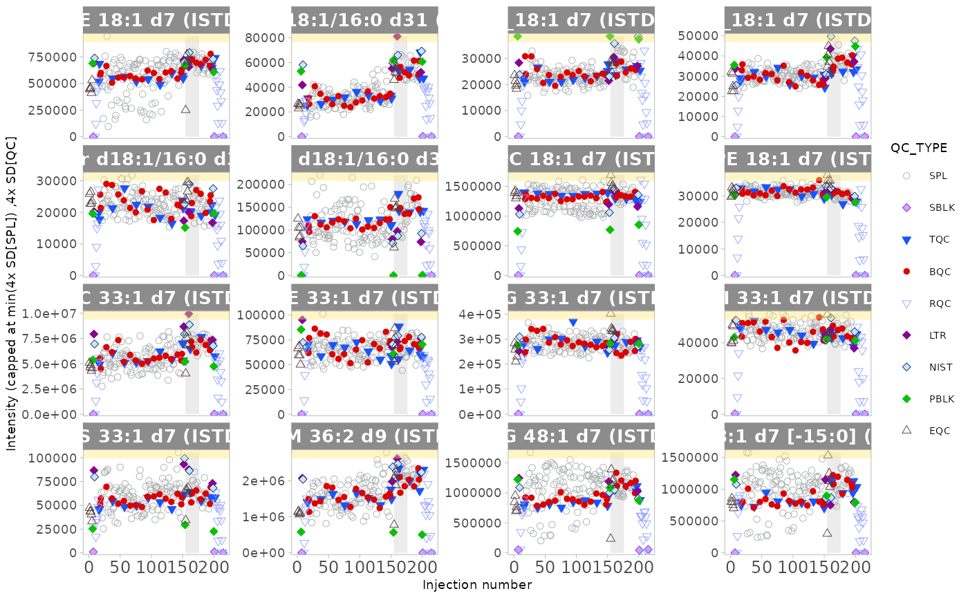
#>  - done!

# Set features QC-filter criteria
 mexp <- filter_features_qc(mexp,
                            max.cv.conc.bqc = 25,
                            min.signalblank.median.spl.pblk = 3,
                            include_qualifier = FALSE,
                            include_istd = FALSE)
#> Calculating feature QC metrics - please wait...
#> ✔ New feature QC filters were defined: 19 of 19 quantifier features meet QC criteria (not including the 9 quantifier ISTD features).

# Save concentration data
 save_dataset_csv( mexp,
                   path = "mydata.csv",
                   variable = "conc",
                   filter_data = TRUE)
#> ✔ Concentration values for 499 analyses and 19 features have been exported to 'mydata.csv'.
Contributor Code of Conduct
Please note that the midar project is released with a Contributor Code of Conduct. By contributing to this project, you agree to abide by its terms.