
Quantitative assay with Ext. calibration and QC
Source:vignettes/articles/recipe-01-ext-calibration-qc.Rmd
recipe-01-ext-calibration-qc.RmdRecipe
This vignette demonstrates a simple workflow for a quantitative targeted assay with external calibration and quality control samples, as used e.g., in clinical chemistry or environmental analysis.
For this type of analysis the known/target concentrations for the
calibrator and QC samples must be defined in the
QCconcentrations metadata. This also requires that
sample_id and analyte_id is defined for the
corresponding analyses in the analysis, and for the features in the
feature metadata tables, respectively.
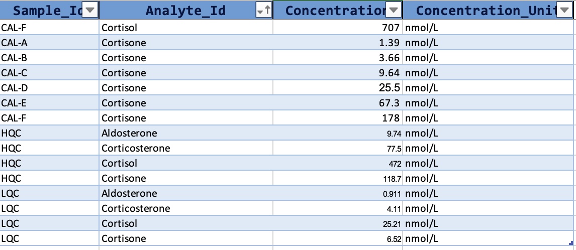
The data and metadata are first imported from a MassHunter CSV file and an MSOrganiser template file. The datasets used in this example can be obtained from https://github.com/SLINGhub/mrmhub/tree/main/data-raw.
library(mrmhub)

# Create a new MRMhubExperiment data object
mexp <- MRMhubExperiment(title = "Corticosteroid Assay")

# Import analysis data (peak integration results) from a MassHunter CSV file
mexp <- import_data_masshunter(
  data = mexp,
  path = "QuantLCMS_Example_MassHunter.csv",
  import_metadata = TRUE)
#> Warning: ! Unrecognized qc_type value(s): "Cal".
#> ℹ These are not standard QC types and may be dropped from QC metrics and plots
#>   that expect them.
#> ℹ Standard values: "SBLK", "TBLK", "UBLK", "HQC", "MQC", "LQC", "QC", "PBLK",
#>   "CAL", "EQA", "PQC", "TQC", "BQC", "RQC", "EQC", "NIST", "LTR", "SPL", "SST",
#>   and "MBLK" ("Sample" is an alias for "SPL").

# Import metadata from an MSOrganiser template file
mexp <- import_metadata_msorganiser(
  mexp,
  path = "datasets/QuantLCMS_Example_MetadataTemplate.xlsx",
  excl_unmatched_analyses = TRUE, ignore_warnings = TRUE)
#> Warning: ! Unrecognized qc_type value(s): "IBLK".
#> ℹ These are not standard QC types and may be dropped from QC metrics and plots
#>   that expect them.
#> ℹ Standard values: "SBLK", "TBLK", "UBLK", "HQC", "MQC", "LQC", "QC", "PBLK",
#>   "CAL", "EQA", "PQC", "TQC", "BQC", "RQC", "EQC", "NIST", "LTR", "SPL", "SST",
#>   and "MBLK" ("Sample" is an alias for "SPL").
#> --------------------------------------------------------------------------------
#> # A tibble: 1 × 5
#>   Type  Table    Column    Issue                        Count
#>   <chr> <chr>    <chr>     <chr>                        <int>
#> 1 N     Analyses sample_id Not defined for all analyses     8
#>
#> --------------------------------------------------------------------------------
#> E = Error, W = Warning, W* = Suppressed Warning, N = Note
#> --------------------------------------------------------------------------------
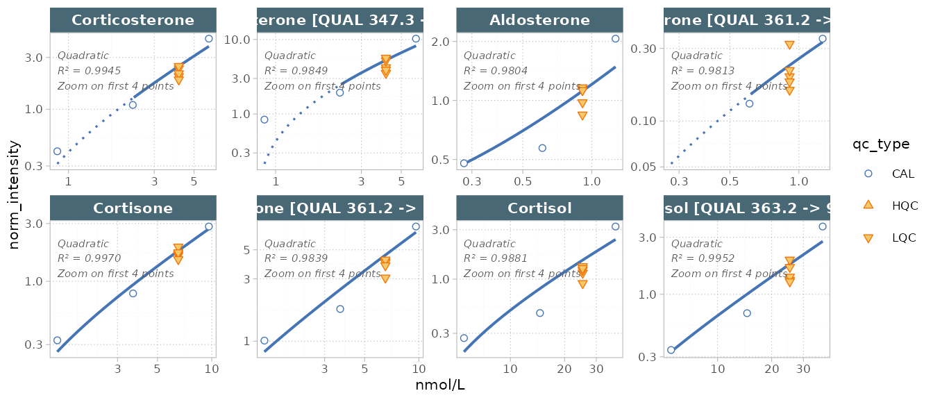
Next, the raw peak areas are normalized with the corresponding internal standard, and the regression fits for the external calibration curves are then calculated and plotted.
# Normalize data by internal standards (defined in feature metadata)
mexp <- normalize_by_istd(mexp)

# Calculate calibration results. The regression model and weighting
# can also be specified per feature in the feature metadata
mexp <- calc_calibration_results(
  mexp,
  fit_overwrite  = TRUE,  # Set to FALSE if defined in metadata
  fit_model = "quadratic",
  fit_weighting = "1/x")

# Plot calibration curves
  plot_calibrationcurves(
    data = mexp, zoom_n_points = 4,
    fit_overwrite = TRUE,  # Set to FALSE if defined in metadata
    fit_model = "quadratic",
    fit_weighting = "1/x",log_scale = TRUE,
    rows_page = 2,
    cols_page = 4, show_progress = FALSE
  )
A summary of the calibration curve results can also be produced:
tbl_cal <- get_calibration_metrics(mexp)
tbl_cal
#> # A tibble: 8 × 14
#>   feature_id   is_quantifier fit_model fit_weighting reg_failed    r2 lowest_cal
#>   <chr>        <lgl>         <chr>     <chr>         <lgl>      <dbl>      <dbl>
#> 1 Aldosterone  TRUE          quadratic 1/x           FALSE      0.980      0.277
#> 2 Aldosterone… FALSE         quadratic 1/x           FALSE      0.981      0.277
#> 3 Corticoster… TRUE          quadratic 1/x           FALSE      0.994      2.28
#> 4 Corticoster… FALSE         quadratic 1/x           FALSE      0.985      2.28
#> 5 Cortisol     TRUE          quadratic 1/x           FALSE      0.988      5.52
#> 6 Cortisol [Q… FALSE         quadratic 1/x           FALSE      0.995      5.52
#> 7 Cortisone    TRUE          quadratic 1/x           FALSE      0.997      1.39
#> 8 Cortisone [… FALSE         quadratic 1/x           FALSE      0.984      1.39
#> # ℹ 7 more variables: highest_cal <dbl>, coef_a <dbl>, coef_b <dbl>,
#> #   coef_c <dbl>, lod <dbl>, loq <dbl>, sigma <dbl>
The summary includes the limit of detection (lod) and
limit of quantification (loq) for each feature, calculated
following the ICH Q2(R1/R2) approach (LoD = 3.3 σ / S, LoQ = 10 σ / S),
where σ is the residual standard error of the regression and S is the
slope of the calibration curve at zero concentration (the linear
coefficient; the quadratic term does not contribute to this slope).
Once the curves have been inspected and the quality of the analysis is satisfactory, the concentrations for all features in samples can be calculated using the external calibration curves.
A summary of the QC results (bias and variability) is calculated and shown below. The final concentration data is saved to a CSV file.
# Calculate concentrations for all samples using external calibration
mexp <- quantify_by_calibration(
  mexp,
  fit_overwrite = FALSE,
  include_qualifier = FALSE,
  ignore_failed_calibration = TRUE,
  fit_model = "quadratic",
  fit_weighting = "1/x")

# get a table with QC results (bias and variability)
tbl <- get_qc_bias_variability(mexp, qc_types = c("HQC", "LQC"))

# Save a table with final concentration data
 save_dataset_csv( mexp,
                   path = "corticosteroid_conc.csv",
                   variable = "conc",
                   filter_data = FALSE)

 print(tbl)
#> # A tibble: 8 × 10
#>   feature_id     sample_id qc_type     n conc_target conc_mean conc_sd cv_intra
#>   <chr>          <chr>     <chr>   <int>       <dbl>     <dbl>   <dbl>    <dbl>
#> 1 Aldosterone    HQC       HQC         5       9.74      8.65    1.14     13.1
#> 2 Aldosterone    LQC       LQC         5       0.911     0.843   0.132    15.7
#> 3 Corticosterone HQC       HQC         5      77.5      75.5     2.98      3.95
#> 4 Corticosterone LQC       LQC         5       4.11      3.64    0.378    10.4
#> 5 Cortisol       HQC       HQC         5     472       495.     68.3      13.8
#> 6 Cortisol       LQC       LQC         5      25.2      20.0     2.40     12.0
#> 7 Cortisone      HQC       HQC         5     119.      114.      6.73      5.89
#> 8 Cortisone      LQC       LQC         5       6.52      6.23    0.504     8.08
#> # ℹ 2 more variables: bias <dbl>, frac_conc_out_of_range <dbl>
Next steps
- Calibration by a Reference Sample — an alternative to external calibration curves
- Custom QC Report — build a formatted QC report from processed data
- Visualisation Functions — the plotting reference, including calibration and QC plots