Correcting isotopic interference

Tutorial Prerequisites: Full workflow

MRMhub corrects isotopic (M+2) overlap between co-eluting same-class lipids with LICAR (Gao et al. 2021). It runs on the raw feature_intensity and, unlike drift and batch correction, applies to every sample. This tutorial annotates the pattern, derives the overlaps, inspects them, and subtracts them; the Isotopic interference correction manual covers the concepts, the derivation levels, and the full mrm_pattern list.

1. Annotate the MRM pattern

Automatic derivation needs one hand-added column, mrm_pattern, on the Features metadata sheet; it names the lipid class and the product-ion type (the manual lists every label and shows the column in context). The valid labels for a product-ion type are returned by licar_pattern_choices():

library(mrmhub)
licar_pattern_choices("Head Group")

MRMhub validates the label on import. Load a processed object to continue:

mexp <- readRDS("results/mexp_processed.rds")

2. Derive the interference relationships

calc_isotopic_interferences() discovers the M+2 overlaps and stores them in annot_interferences. Set level = "MRM" for class-based LC-MRM; "MS1" is only for genuine full-scan data, not a fallback when a product m/z is missing (see the manual).

# Class-based LC-MRM: fragment-level M+2 (needs precursor + product m/z).
mexp <- calc_isotopic_interferences(mexp, level = "MRM")

# Genuine MS1 / full-scan: whole-molecule M+2 (needs precursor m/z only).
# mexp <- calc_isotopic_interferences(mexp, level = "MS1")

Derivation is deterministic; raise min_contribution to drop negligible pairs.

3. Inspect the derived relationships

Before subtracting, review the derived overlaps. Each row of annot_interferences is one overlap, described by its overlap_type and source columns (defined in the manual):

mexp@annot_interferences

summarize_interferences() rolls this up per feature: how many are affected, split by source and overlap type, with the contribution-factor range.

summarize_interferences(mexp)

4. Apply the correction

correct_isotopic_interferences() subtracts all derived overlaps from the raw intensities in one pass (its reference page gives the formula and zero-clamping).

mexp <- correct_isotopic_interferences(mexp)

Apply it before ISTD normalisation, drift, and batch correction; running it later resets those steps (with a warning). Uncorrected values are kept in feature_intensity_orig. Overlaps you annotate yourself (in-source fragments, co-eluting isobars) are applied with correct_custom_interferences().

5. Correct a single pair manually

For a one-off correction, or to check a factor before trusting the automatic derivation, use correct_interference_manual(), where variable is the dataset column:

mexp <- correct_interference_manual(
  mexp,
  variable = "feature_intensity",
  feature = "PC 32:0",
  interfering_feature = "SM 36:1 M+3",
  interference_contribution = 0.0107,
  neg_to_na = FALSE,
  updated_feature_id = NA)

updated_feature_id renames the corrected feature so the raw and corrected channels can coexist.

6. Verify the correction

Compare a corrected feature’s intensities before and after; in blanks (SBLK/PBLK) the residual signal should approach zero, and a non-zero blank median points to an underestimated factor.

d <- get_analyticaldata(mexp, annotated = TRUE) |>
  dplyr::filter(feature_id == "PC 32:0") |>
  dplyr::select(
    analysis_id, qc_type,
    intensity_before = feature_intensity_orig,
    intensity_after = feature_intensity) |>
  dplyr::mutate(
    pct_change =
      100 * (intensity_after - intensity_before) / intensity_before)

summary(d$pct_change)

plot_qc_interference_impact() shows how many features were corrected at each magnitude (percent of signal removed):

plot_qc_interference_impact(mexp, qc_types = "SPL")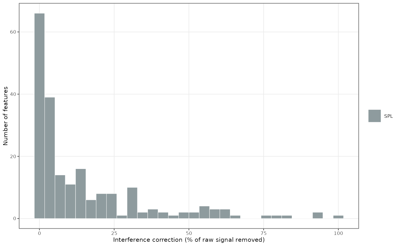

Figure 1. How many features were corrected at each magnitude (percent of signal removed) in the study samples.

plot_interference_correction() plots each feature’s residual signal as a percent of its uncorrected value, split by QC type. min_correction_pct restricts it to strongly affected features (here ≥ 40 % removed), sort_by_effect ranks by magnitude, and top_n keeps the largest:

plot_interference_correction(
  mexp,
  qc_types = "SPL",
  min_correction_pct = 40,
  sort_by_effect = "desc",
  point_size = 1.5, point_alpha = 0.8)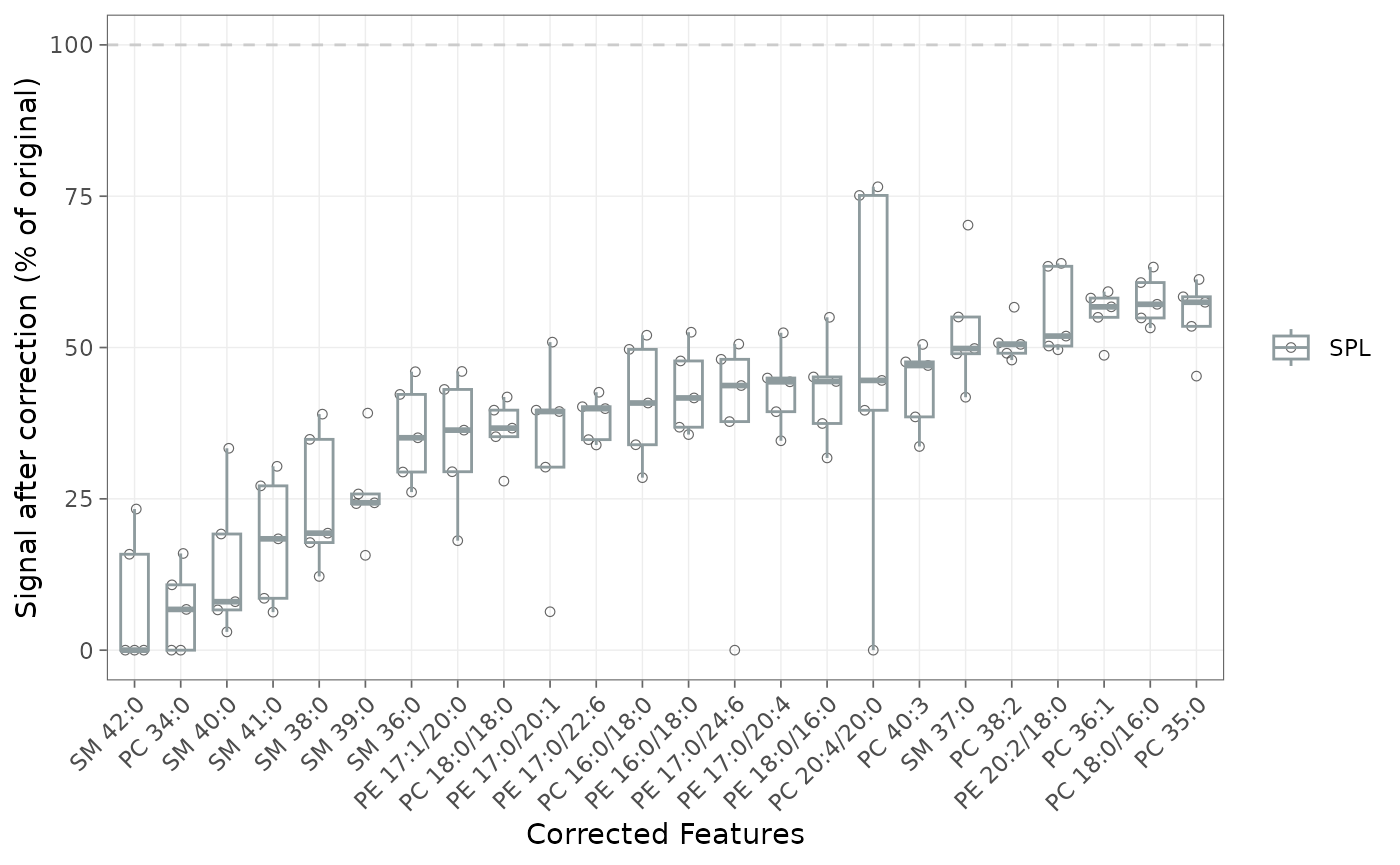

Figure 2. Per-feature residual signal after correction, as a percent of the uncorrected value, for features with at least 40% removed, split by QC type.

Co-elution filtering (experimental)

check_coelution is experimental and off by default. Verify the pairs it keeps and drops on your own data before relying on it.

The correction subtracts the full source area, so it is valid only where the source and target peaks co-elute and/or are co-integrated. The experimental check_coelution gate keeps only the m/z-matched edges that pass this test and drops chromatographically resolved pairs (see the manual):

mexp <- calc_isotopic_interferences(
  mexp, level = "MRM", check_coelution = TRUE)

It is off by default while the gate is validated, and reports how many pairs it drops.

Next steps

• Isotopic interference correction (manual): concepts, derivation levels, and the full label list
• Drift and batch correction: apply after interference correction
• Lipidomics workflow: the full processing pipeline
• The MRMhubExperiment data object: how _orig preserves the raw intensities

References

Gao, Liang, Shanshan Ji, Bo Burla, Markus R. Wenk, Federico Torta, and Amaury Cazenave-Gassiot. 2021. “LICAR: An Application for Isotopic Correction of Targeted Lipidomic Data Acquired with Class-Based Chromatographic Separations Using Multiple Reaction Monitoring.” Analytical Chemistry 93 (6): 3163–71. https://doi.org/10.1021/acs.analchem.0c04565.