
Quantification with external calibration
Source:vignettes/articles/tutorial-06-external-calibration.Rmd
tutorial-06-external-calibration.RmdExternal calibration quantifies each analyte from a calibration curve measured alongside the samples, as used in clinical chemistry, toxicology and environmental analysis. This tutorial fits one curve per analyte from a dilution series of calibrators, quantifies the samples, and checks the result against QC samples with assigned target concentrations. The example is a 15-analyte serum steroid panel measured by LC-MRM-MS, with calibrants (Cal A–F), low and high QCs (LQC, HQC), and external quality-assessment samples in place of study samples.
The target concentrations for the calibrators and QCs live in the
QCconcentrations metadata, which requires
sample_id in the analysis metadata and
analyte_id in the feature metadata.
The full, reproducible report for this dataset (including drift-range flags, exports and the underlying data) is published as Dataset 4 in the MRMhub-workflows supplement.
1. Import data and metadata
We load the INTEGRATOR peak areas into a fresh
MRMhubExperiment, then attach the metadata workbook that
defines the analytes, their internal standards, the sample annotations,
and the calibration and target concentrations.
library(mrmhub)

mexp <- MRMhubExperiment(title = "Steroid Assay")
mexp <- import_data_mrmhub(
  mexp,
  path = "datasets/Dataset4_MRMhub-INTEGRATOR_ASSAY.csv",
  import_metadata = TRUE)
✔ Imported 20 analyses with 64 features.ℹ feature_area selected as default feature intensity. Modify with `set_intensity_var()`.✔ Analysis metadata associated with 20 analyses.✔ Feature metadata associated with 64 features.mexp <- import_metadata_msorganiser(
mexp,
path = "datasets/Dataset4_Metadata.xlsx",
excl_unmatched_analyses = TRUE,
ignore_warnings = TRUE)
Found no errors, 2 warnings, and 2 notes in the metadata.
----------------------------------------------------------------
Type Table Column Issue Count
1 W* Analyses analysis_id Analyses not in analysis data 12
2 W* Features feature_id Feature(s) without metadata 34
3 N Analyses sample_id Not defined for all analyses 16
4 N Features analyte_id Not defined for all features 15
----------------------------------------------------------------
E = Error, W = Warning, W* = Suppressed Warning, N = Note
----------------------------------------------------------------✔ Analysis metadata associated with 20 analyses.✔ Feature metadata associated with 30 features.✔ Internal Standard metadata associated with 15 ISTDs.✔ QC concentration metadata associated with 13 samples and 15 analytes2. Fit the calibration curves
normalize_by_istd() divides each analyte’s peak area by
that of its internal standard, writing the ratio to
feature_norm_intensity.
calc_calibration_results() then fits one curve per analyte
from the calibrator levels (here a quadratic model with 1/x
weighting for all analytes). The model and weighting can also be set per
analyte in the feature metadata.
mexp <- normalize_by_istd(mexp)✔ 15 features normalized with 15 ISTDs in 20 analyses.
mexp <- calc_calibration_results(
  mexp,
  fit_overwrite = TRUE,
  fit_model = "quadratic",
  fit_weighting = "1/x")
✔ Calibration curve fits calculated for all 15 quantifier features. Average r²: 0.9978.Inspect the fitted curves before quantifying: each analyte’s response should rise steadily across the calibrator range and fit the points well, and the samples should fall inside that range rather than on the dotted, extrapolated section.
plot_calibrationcurves(
  mexp,
  fit_overwrite = TRUE,
  fit_model = "quadratic",
  fit_weighting = "1/x",
  include_istd = FALSE,
  include_qualifier = FALSE,
  rows_page = 4, cols_page = 4,
  show_progress = FALSE)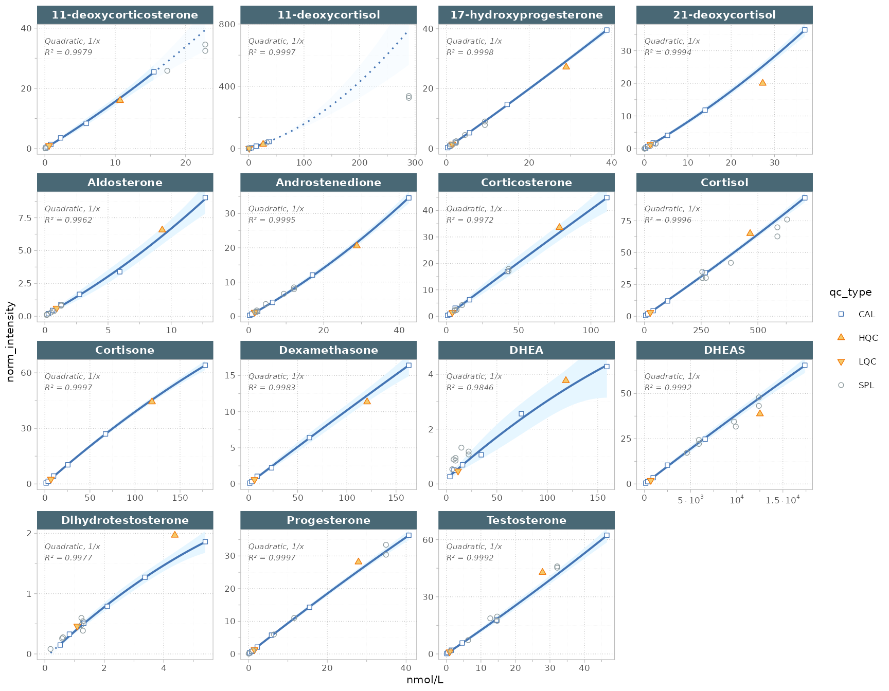
Figure 1. Quadratic, 1/x-weighted calibration curves for the 15 steroid analytes. Curves are solid within the calibrator range and dotted where extrapolated.
get_calibration_metrics() summarises each fit: the R²
for linearity and the limits of detection and quantification
(lod, loq), in the calibrated concentration
unit.
get_calibration_metrics(
  mexp,
  include_qualifier = FALSE, summary_table = TRUE)
# A tibble: 15 × 6
   analyte                fit_model fit_weighting    r2   lod    loq
   <chr>                  <chr>     <chr>         <dbl> <dbl>  <dbl>
 1 11-deoxycorticosterone quadratic 1/x           0.998 0.457  1.38
 2 11-deoxycortisol       quadratic 1/x           1.000 0.279  0.844
 3 17-hydroxyprogesterone quadratic 1/x           1.000 0.197  0.596
 4 21-deoxycortisol       quadratic 1/x           0.999 0.427  1.29
 5 Aldosterone            quadratic 1/x           0.996 0.639  1.94
 6 Androstenedione        quadratic 1/x           0.999 0.445  1.35
 7 Corticosterone         quadratic 1/x           0.997 1.25   3.79
 8 Cortisol               quadratic 1/x           1.000 1.22   3.71
 9 Cortisone              quadratic 1/x           1.000 0.463  1.4
10 DHEA                   quadratic 1/x           0.985 3.03   9.18
11 DHEAS                  quadratic 1/x           0.999 8.29  25.1
12 Dexamethasone          quadratic 1/x           0.998 1.19   3.6
13 Dihydrotestosterone    quadratic 1/x           0.998 0.178  0.54
14 Progesterone           quadratic 1/x           1.000 0.251  0.76
15 Testosterone           quadratic 1/x           0.999 0.458  1.39
3. Quantify the samples
Once the curves are satisfactory,
quantify_by_calibration() inverts each fitted curve to
convert the normalized intensities into absolute concentrations, written
to feature_conc. Using
ignore_failed_calibration = TRUE skips any analyte whose
curve failed to fit rather than aborting the whole run.
mexp <- quantify_by_calibration(
  mexp,
  fit_overwrite = FALSE,
  include_qualifier = FALSE,
  ignore_failed_calibration = TRUE,
  fit_model = "quadratic",
  fit_weighting = "1/x")
✔ Calibration curve fits calculated for all 15 quantifier features. Average r²: 0.9978.ℹ 77 concentration values fall outside the calibrated range (retained, flagged in feature_conc_out_of_range).✔ Concentrations calculated for 15 features in 20 analyses.✔ Concentrations are given in nmol/L.4. Check QC bias and variability
The final check compares the measured QC concentrations against their
known targets. get_qc_bias_variability() reports, per
analyte and QC level, the mean measured concentration, the
bias (percent deviation from target, i.e. accuracy) and
the intra-batch %CV (precision).
get_qc_bias_variability(
  mexp,
  qc_types = c("LQC", "HQC"), summary_table = TRUE)
# A tibble: 30 × 9
   feature_id      sample_id qc_type     n conc_target conc_mean cv_intra   bias
   <chr>           <chr>     <chr>   <int>       <dbl>     <dbl>    <dbl>  <dbl>
 1 11-deoxycortic… LQC       LQC         1       0.593     0.672       NA  13.4
 2 11-deoxycortic… HQC       HQC         1      10.7      10.2         NA  -4.68
 3 11-deoxycortis… LQC       LQC         1       1.38      1.45        NA   5.3
 4 11-deoxycortis… HQC       HQC         1      26.5      23.5         NA -11.3
 5 17-hydroxyprog… LQC       LQC         1       1.42      1.51        NA   6.57
 6 17-hydroxyprog… HQC       HQC         1      29        27.1         NA  -6.61
 7 21-deoxycortis… LQC       LQC         1       1.38      1.68        NA  21.7
 8 21-deoxycortis… HQC       HQC         1      27.3      22.4         NA -18
 9 Aldosterone     LQC       LQC         1       0.929     0.988       NA   6.33
10 Aldosterone     HQC       HQC         1       9.29      9.86        NA   6.18
# ℹ 20 more rows
# ℹ 1 more variable: frac_conc_out_of_range <dbl>
For a quantitative assay, bias and CV within roughly ±15% (±20% near the quantification limit) is a common acceptance guide, though the exact limits depend on the application and any regulatory requirements.
5. Export the concentrations
save_dataset_csv() writes a flat table of
concentrations, one row per sample. add_qctype = TRUE keeps
the QC-type column so calibrators, QCs and samples stay distinguishable.
For a multi-sheet workbook that also bundles the calibration and QC
metrics, use save_report_xlsx().
save_dataset_csv(
  mexp,
  path = "steroid_conc.csv",
  variable = "conc",
  add_qctype = TRUE)
Next steps
- Calibration by a reference sample: an alternative when no calibration series is available
- Visualisation functions: the plotting reference, including calibration and QC plots