Here is an example to output plot in ggplot2 into
trellis. The example in plotly can be found in vignette
“Plots in plotly”.
library(lancer)

# Data Creation

concentration <- c(
  10, 20, 25, 40, 50, 60,
  75, 80, 100, 125, 150,
  10, 25, 40, 50, 60,
  75, 80, 100, 125, 150
)

curve_batch_name <- c(
  "B1", "B1", "B1", "B1", "B1",
  "B1", "B1", "B1", "B1", "B1", "B1",
  "B2", "B2", "B2", "B2", "B2",
  "B2", "B2", "B2", "B2", "B2"
)

sample_name <- c(
  "Sample_010a", "Sample_020a",
  "Sample_025a", "Sample_040a", "Sample_050a",
  "Sample_060a", "Sample_075a", "Sample_080a",
  "Sample_100a", "Sample_125a", "Sample_150a",
  "Sample_010b", "Sample_025b",
  "Sample_040b", "Sample_050b", "Sample_060b",
  "Sample_075b", "Sample_080b", "Sample_100b",
  "Sample_125b", "Sample_150b"
)

curve_1_saturation_regime <- c(
  5748124, 16616414, 21702718, 36191617,
  49324541, 55618266, 66947588, 74964771,
  75438063, 91770737, 94692060,
  5192648, 16594991, 32507833, 46499896,
  55388856, 62505210, 62778078, 72158161,
  78044338, 86158414
)

curve_2_good_linearity <- c(
  31538, 53709, 69990, 101977, 146436, 180960,
  232881, 283780, 298289, 344519, 430432,
  25463, 63387, 90624, 131274, 138069,
  205353, 202407, 260205, 292257, 367924
)

curve_3_noise_regime <- c(
  544, 397, 829, 1437, 1808, 2231,
  3343, 2915, 5268, 8031, 11045,
  500, 903, 1267, 2031, 2100,
  3563, 4500, 5300, 8500, 10430
)

curve_4_poor_linearity <- c(
  380519, 485372, 478770, 474467, 531640, 576301,
  501068, 550201, 515110, 499543, 474745,
  197417, 322846, 478398, 423174, 418577,
  426089, 413292, 450190, 415309, 457618
)

curve_batch_annot <- tibble::tibble(
  Sample_Name = sample_name,
  Curve_Batch_Name = curve_batch_name,
  Concentration = concentration
)

curve_data <- tibble::tibble(
  Sample_Name = sample_name,
  `Curve_1` = curve_1_saturation_regime,
  `Curve_2` = curve_2_good_linearity,
  `Curve_3` = curve_3_noise_regime,
  `Curve_4` = curve_4_poor_linearity
)

curve_table <- lancer::create_curve_table(
  curve_batch_annot = curve_batch_annot,
  curve_data_wide = curve_data,
  common_column = "Sample_Name",
  signal_var = "Signal",
  column_group = "Curve_Name"
)

curve_classified <- curve_table |>
  lancer::summarise_curve_table(
    grouping_variable = c(
      "Curve_Name",
      "Curve_Batch_Name"
    ),
    conc_var = "Concentration",
    signal_var = "Signal"
  ) |>
  dplyr::arrange(.data[["Curve_Name"]]) |>
  lancer::evaluate_linearity(
    grouping_variable = c(
      "Curve_Name",
      "Curve_Batch_Name"
  ))
Here is the output of curve_table and
curve_classified
print(head(curve_table), width = 100)
#> # A tibble: 6 × 5
#>   Sample_Name Curve_Batch_Name Concentration Curve_Name   Signal
#>   <chr>       <chr>                    <dbl> <chr>         <dbl>
#> 1 Sample_010a B1                          10 Curve_1     5748124
#> 2 Sample_010a B1                          10 Curve_2       31538
#> 3 Sample_010a B1                          10 Curve_3         544
#> 4 Sample_010a B1                          10 Curve_4      380519
#> 5 Sample_020a B1                          20 Curve_1    16616414
#> 6 Sample_020a B1                          20 Curve_2       53709
print(head(curve_classified), width = 100)
#> # A tibble: 6 × 11
#>   Curve_Name Curve_Batch_Name wf1_group      wf2_group         r_corr pra_linear
#>   <chr>      <chr>            <chr>          <chr>              <dbl>      <dbl>
#> 1 Curve_1    B1               Poor Linearity Saturation Regime  0.963       70.5
#> 2 Curve_1    B2               Poor Linearity Saturation Regime  0.950       62.3
#> 3 Curve_2    B1               Good Linearity Good Linearity     0.990       92.8
#> 4 Curve_2    B2               Good Linearity Good Linearity     0.995       94.3
#> 5 Curve_3    B1               Poor Linearity Noise Regime       0.964       71.2
#> 6 Curve_3    B2               Poor Linearity Noise Regime       0.978       74.7
#>   mandel_p_val concavity r2_linear r2_adj_linear mandel_stats
#>          <dbl>     <dbl>     <dbl>         <dbl>        <dbl>
#> 1   0.0000297  -4174.        0.928         0.920       71.2
#> 2   0.000166   -4137.        0.903         0.890       52.9
#> 3   0.150         -4.91      0.980         0.978        2.53
#> 4   0.382         -1.94      0.990         0.988        0.868
#> 5   0.00000678     0.468     0.930         0.922      106.
#> 6   0.00256        0.321     0.956         0.951       20.9
We then create the ggplot plots with
curve_table and curve_classified
# Create a trellis table
trellis_table_orig <- lancer::add_ggplot_panel(
  curve_table = curve_table,
  curve_summary = curve_classified,
  grouping_variable = c(
    "Curve_Name",
    "Curve_Batch_Name"
  ),
  curve_batch_var = "Curve_Batch_Name",
  curve_batch_col = c(
    "#377eb8",
    "#4daf4a"
  ),
  conc_var = "Concentration",
  conc_var_units = "%",
  conc_var_interval = 50,
  signal_var = "Signal",
  plot_first_half_lin_reg = FALSE
)

trellis_list_orig <- trellis_table_orig$panel
To output these plots as a trellis in html, convert the
grouping_variable as conditional variable, the
column holding the plots as a panel_variable and the other
columns as common cognostics.
We use the function convert_to_cog which uses the
default cog_df created by
create_default_cog_df.
lancer::create_default_cog_df()
#>        col_name_vec                                    desc_vec type_vec
#> 1        Curve_Name                                  Curve_Name   factor
#> 2  Curve_Batch_Name                            Curve_Batch_Name   factor
#> 3       Curve_Class                           Classes of Curves   factor
#> 4         wf1_group                       Group from workflow 1   factor
#> 5         wf2_group                       Group from workflow 2   factor
#> 6            r_corr                Pearson Correlation R values  numeric
#> 7        pra_linear Linear Regression Percent Residual Accuracy  numeric
#> 8      mandel_p_val                    P values for Mandel test  numeric
#> 9         r2_linear                 Linear Regression R^2 Value  numeric
#> 10    r2_adj_linear        Linear Regression Adjusted R^2 Value  numeric
#> 11     mandel_stats             Test statistics for Mandel Test  numeric
#> 12        adl_value            Average Deviation from Linearity  numeric
Using the function convert_to_cog,
trellis_table_convert <- trellis_table_orig |>
  lancer::convert_to_cog(
    grouping_variable = c(
      "Curve_Name",
      "Curve_Batch_Name"
    ),
    panel_variable = "panel"
  )
The output is as follows.
print(head(trellis_table_convert), width = 100)
#> # A tibble: 6 × 12
#>   Curve_Name Curve_Batch_Name wf1_group      wf2_group       r_corr   pra_linear
#>   <cog>      <cog>            <cog>          <cog>           <cog>    <cog>
#> 1 Curve_1    B1               Poor Linearity Saturation Reg… 0.963362   70.49412
#> 2 Curve_2    B1               Good Linearity Good Linearity  0.989903   92.75456
#> 3 Curve_3    B1               Poor Linearity Noise Regime    0.964252   71.18372
#> 4 Curve_4    B1               Poor Linearity Poor Linearity  0.311458 -251.44937
#> 5 Curve_1    B2               Poor Linearity Saturation Reg… 0.950007   62.30351
#> 6 Curve_2    B2               Good Linearity Good Linearity  0.994815   94.32046
#>   mandel_p_val concavity     r2_linear r2_adj_linear mandel_stats panel
#>   <cog>        <cog>         <cog>     <cog>         <cog>        <trllscp_>
#> 1 2.968599e-05 -4174.1333061 0.928067   0.920074      71.2051525  <patchwrk>
#> 2 1.501138e-01    -4.9071785 0.979908   0.977675       2.5335524  <patchwrk>
#> 3 6.775079e-06     0.4677827 0.929783   0.921981     106.2121740  <patchwrk>
#> 4 6.599208e-03   -20.5225862 0.097006  -0.003327      13.2417851  <patchwrk>
#> 5 1.662149e-04 -4136.5254757 0.902514   0.890328      52.9344641  <patchwrk>
#> 6 3.824145e-01    -1.9381407 0.989657   0.988364       0.8684023  <patchwrk>
Observe that the attributes of the columns are different. For the grouping variable column labelled we have
print(attributes(trellis_table_convert$Curve_Name))
#> $cog_attrs
#> $cog_attrs$desc
#> [1] "conditioning variable"
#>
#> $cog_attrs$type
#> [1] "factor"
#>
#> $cog_attrs$group
#> [1] "condVar"
#>
#> $cog_attrs$defLabel
#> [1] TRUE
#>
#> $cog_attrs$defActive
#> [1] TRUE
#>
#> $cog_attrs$filterable
#> [1] TRUE
#>
#> $cog_attrs$log
#> [1] NA
#>
#>
#> $class
#> [1] "cog"       "character"
For the column labelled as a panel_variable, we have
print(attributes(trellis_table_convert$panel))
#> $class
#> [1] "trelliscope_panels" "list"
For the rest of the column converted to a common cognostics, we have
print(attributes(trellis_table_convert$r_corr))
#> $cog_attrs
#> $cog_attrs$desc
#> [1] "Pearson Correlation R values"
#>
#> $cog_attrs$type
#> [1] "numeric"
#>
#> $cog_attrs$group
#> [1] "common"
#>
#> $cog_attrs$defLabel
#> [1] FALSE
#>
#> $cog_attrs$defActive
#> [1] TRUE
#>
#> $cog_attrs$filterable
#> [1] TRUE
#>
#> $cog_attrs$log
#> [1] NA
#>
#>
#> $class
#> [1] "cog"     "numeric"
It is also possible for users to create their own cognostics as well.
curve_name <- c("Curve_1", "Curve_2", "Curve_3", "Curve_4")
curve_class <- c("Class_1", "Class_1", "Class_2", "Class_2")
curve_name_annot <- tibble::tibble(
Curve_Name = curve_name,
Curve_Class = curve_class
)
col_name_vec <- c("Curve_Name", "Curve_Class")
desc_vec <- c(
"Names of Curves",
"Classes of Curves"
)
type_vec <- c("factor", "factor")
cog_df <- data.frame(
col_name_vec = col_name_vec,
desc_vec = desc_vec,
type_vec = type_vec
)
trellis_table_orig_converted <- trellis_table_orig |>
dplyr::left_join(curve_name_annot, by = "Curve_Name") |>
lancer::convert_to_cog(
cog_df = cog_df,
grouping_variable = c(
col_name_vec,
"Curve_Batch_Name"
),
panel_variable = "panel",
col_name_vec = "col_name_vec",
desc_vec = "desc_vec",
type_vec = "type_vec"
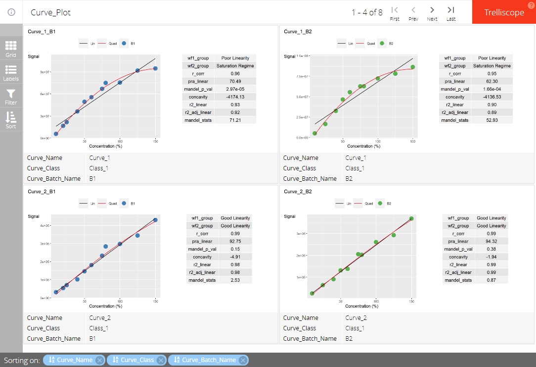
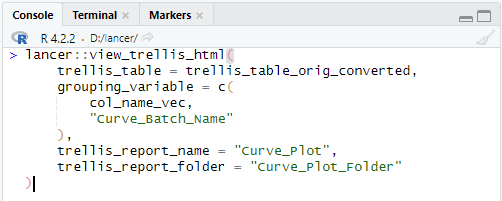
)The list of ggplots can be output as follows by calling
this command in the R console:
lancer::view_trellis_html(
  trellis_table = trellis_table_orig_converted,
  grouping_variable = c(
    col_name_vec,
    "Curve_Batch_Name"
  ),
  trellis_report_name = "Curve_Plot",
  trellis_report_folder = "Curve_Plot_Folder"
)
This will create a folder called “Curve_Plot_Folder” as defined by
trellis_report_folder in your current working
directory.
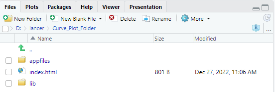
You may view the plots by clicking on “index.html”